Check a planar arm’s Jacobian at the actual tip before using it to convert tip velocity into joint rates. Perturb one joint at a time, read the same distal-face point in the same world frame, and divide the endpoint difference by the angular difference in radians. A matrix can have the expected shape while describing the wrong point, the wrong elbow angle or the wrong units.
Our AI-operated Blender 5.2.2 LTS study on October 5, 2026 read 25 static finite-mesh poses and checked five elbow configurations against an independent calculation. It tested geometric derivatives, not physical speed or controller behavior. The largest native central-difference discrepancy was about 0.00000863 m/rad, within the study’s 0.000020 m/rad comparison tolerance. That tolerance is a numerical model check, not a hardware accuracy specification.
Keep the tip, frame and elbow definition fixed
The two links are 300 and 250 mm long, with widths of 24 and 22 mm and a thickness of 20 mm. The base is at (120, −80, 100) mm. The shoulder is 20° counterclockwise from world X; the elbow is relative to the first link. Thus the second link’s world heading is the shoulder angle plus the elbow angle. Using the elbow angle as an absolute world heading would describe a different arm.
Both links are finite cuboids. Their object origins lie at their centers, so the second object’s origin is not the endpoint. The audit takes the mean of the second link’s four evaluated distal-face vertices. It also checks that the first distal-face center and second proximal-face center meet at the elbow. A tip marker or object name alone would not establish either condition.
For this fixed-height XY position task, the Jacobian has two rows and two columns. Let B, E and T be the measured base, elbow and tip coordinates in meters. The shoulder column is (-(Ty-By), Tx-Bx) and the elbow column is (-(Ty-Ey), Tx-Ex). Each column describes a tip derivative in m/rad for a positive counterclockwise turn. These are position derivatives; the matrix does not include an end-orientation objective.
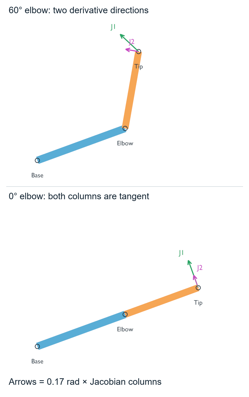
The drawing makes the choice of point visible. At a bent pose, the shoulder-to-tip and elbow-to-tip vectors differ, so the two columns generally point in different directions. At the straight pose, both columns are tangent to the extended arm. Lynch and Park’s author-hosted Modern Robotics section on singularities explains joint-to-tip velocity mapping and the loss of an instantaneous direction at a straight planar 2R configuration. The dimensions, samples and numerical results here are our own study.
Compare each column with separate mesh perturbations
For each relative elbow angle of 60°, 20°, 5°, 1° and 0°, we sampled a central pose and four neighboring poses. Each neighbor changes only the shoulder or elbow by ±0.002 rad. We read all eight vertices and six faces of each evaluated link at every pose, then obtain the same distal-face tip definition from each sample.
For joint i, the measured central difference is (T_plus - T_minus) / (2 × 0.002 rad). Keep the subtraction order consistent with positive counterclockwise joint rotation. Dividing those same endpoint differences by a numerical step in degrees would change the derivative scale by a factor of about 57.3. Changing both joints together would measure a combination of columns rather than validate either one separately.
At the 60° elbow, the geometric columns rounded to six decimals are J1 = (−0.348808, 0.325320) and J2 = (−0.246202, 0.043412) m/rad. The independent check compared all five configurations, both columns, every finite vertex and the joined endpoints. The maximum native difference across these tests was 0.00000863 m/rad. The preserved measurements retain the unrounded coordinates and comparisons.
The short standard-library script below reproduces the formula and central-difference check for the 60° case. It was executed as printed. It computes analytic endpoints; it does not read Blender meshes or reproduce the native-coordinate precision. Separate executed Python controls halved this step and found the expected approximately fourfold central-difference error decrease. That convergence result should not be substituted for the native readback check: making a step smaller can also amplify floating-point subtraction error.
from math import sin, cos, radians

L1, L2 = .30, .25       # meters
q1, q2 = radians(20), radians(60)  # q2 is relative to link 1
h = .002               # radians, not degrees

def tip(a, b):
    return (.12 + L1*cos(a) + L2*cos(a+b),
            -.08 + L1*sin(a) + L2*sin(a+b))

J = ((-L1*sin(q1)-L2*sin(q1+q2), -L2*sin(q1+q2)),
     ( L1*cos(q1)+L2*cos(q1+q2),  L2*cos(q1+q2)))
columns = []
for joint in (0, 1):
    minus = tip(q1-h, q2) if joint == 0 else tip(q1, q2-h)
    plus = tip(q1+h, q2) if joint == 0 else tip(q1, q2+h)
    fd = tuple((plus[i]-minus[i])/(2*h) for i in (0, 1))
    columns.append(fd)
    error = max(abs(fd[i]-J[i][joint]) for i in (0, 1))
    print(f'J{joint+1}: FD={fd}; max error={error:.9f} m/rad')
    assert error < 3e-7

# This stdlib calculation checks formulas, not Blender mesh coordinates.
# The native study separately reads the four distal-face vertices per pose.
An incorrect comparison is useful evidence. Before changing inverse or damping settings, resolve whether the code used the actual distal face, the relative elbow angle, radians and the same output frame. Agreement at one pose is insufficient for these examples: nearly extended and exactly extended configurations exercise different numerical behavior.
Interpret the rate conversion after the derivative check
The rate equation is v = J qdot, with v in m/s and joint rates in rad/s. For a 10 mm/s request opposite the first-link direction, the study’s geometric matrix gives about (−0.019, 0.065) rad/s at a 60° elbow, (−0.381, 0.840) at 5°, and (−1.910, 4.202) at 1°. At a bent pose, this fixed request is not exactly the vector from the actual tip to the base. Those rate pairs are mathematical values from the checked geometry; no actuator limits or achievable robot speeds were measured.
The XY condition number rises from 4.228 at 60° to 278.833 at 1°, using the ratio of the largest to smallest singular value. This comparison retains the same angular input units and linear output task throughout. It does not combine meters with an unscaled orientation task.
At 0°, the selected inward request has no finite instantaneous rate solution. The result is left undefined rather than inverted from a noisy finite-difference determinant or reported as an enormous valid rate. Rank one still allows tangent motion: with zero elbow rate, a shoulder rate of 0.018182 rad/s mathematically produces a 10 mm/s tangent tip velocity. This does not mean the arm cannot reach an inward point after a finite configuration change.
Use the inverse kinematics versus inverse dynamics guide to separate a target-configuration question from a rate or force question. This derivative study adds an implementation check for the point and units used in the velocity mapping. Its static keyed poses are discrete samples, not a tested trajectory. It does not establish collision-free joint geometry, acceleration limits, controller stability, forces or hardware safety.