Short servo moves: raising the speed limit may change nothing

A move that starts and finishes at rest may need to begin braking before it reaches its speed limit. Raising that limit then changes nothing. In the simple position-profile calculation below, a 20° move takes 0.816 s with either a 60°/s or a 120°/s ceiling, because both trajectories peak at only 48.990°/s.

That is a useful possibility to check when a short position move does not become faster after increasing a velocity setting. It is not a diagnosis of every slow servo: these examples prescribe equal acceleration and deceleration of 120°/s², zero starting and finishing speed, and no jerk limit. Motor torque, load, feedback and communication are not modeled.

There is not enough travel for a cruise segment

At 120°/s², reaching 60°/s takes 0.5 s and covers 15°. Stopping from that speed needs another 15°. A move therefore needs 30° of travel just to reach the ceiling and brake, with no time left at constant speed.

Our 20° move must turn around sooner in the speed profile. It accelerates for about 0.408 s, then decelerates for the same time. Doubling the ceiling cannot add travel between the same endpoints, so the peak and duration stay unchanged. The two position-versus-time curves are identical in this model.

The transition matters. At exactly 30°, the profile touches 60°/s and immediately begins braking: total time is 1.000 s, and constant-speed duration is zero. A 120° move with that same ceiling and acceleration has enough room for 1.500 s at 60°/s, giving a total of 2.500 s. Touching the ceiling once and cruising at the ceiling are different outcomes.

For these symmetric rest-to-rest moves, the travel needed to reach a speed ceiling V is V²/a, where a is the acceleration magnitude. Below that travel, the peak is √(aD), where D is the actual travel. Keep the angular units consistent: the calculations here use degrees, degrees per second and degrees per second squared throughout.

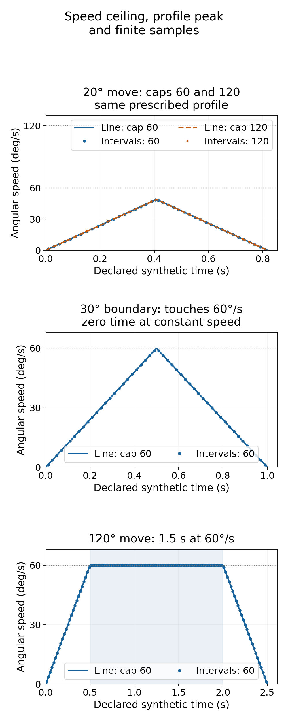
Prescribed travel / cap	Analytic peak	Total time	Cruise time
20° / 60°/s	48.990°/s	0.816 s	0 s
20° / 120°/s	48.990°/s	0.816 s	0 s
30° / 60°/s	60°/s	1.000 s	0 s
120° / 60°/s	60°/s	2.500 s	1.500 s

A profile setting is not a shaft-speed measurement

The ROBOTIS XD540-T150 manual describes Profile Velocity as a maximum velocity when velocity-based profiling is selected. In time-based profiling, that field instead represents a time quantity. The manual’s profile explanation also identifies travel distance as one of the inputs determining the profile type.

Those distinctions support checking the active profile and units before interpreting a setting. Our numbers are not DYNAMIXEL register values, and this calculation does not emulate its firmware, moving-start replanning or tracking behavior. We have not sent commands to a controller or tested a motor.

The scalar comparisons were executed in standalone Python, followed by an AI-operated Blender 5.2.2 LTS study. It set 263 finite poses of a 100 × 12 × 6 mm lever across the four conditions at supplied synthetic times. The final 12-object scene retained the final lever poses, fixed reference wires and measured tip-center traces; raw records preserved all 2,104 pose-vertex rows. An independent audit checked local/world vertices, matrices, faces, normals, sample order and CSV rows, then reconstructed the angles and interval rates. The scene stayed at frame 1: no between-sample animation, controller, firmware or physical motor timing was tested. The 0.0002° angle and 0.02°/s interval comparison allowances check numerical readback; they do not establish actuator accuracy.

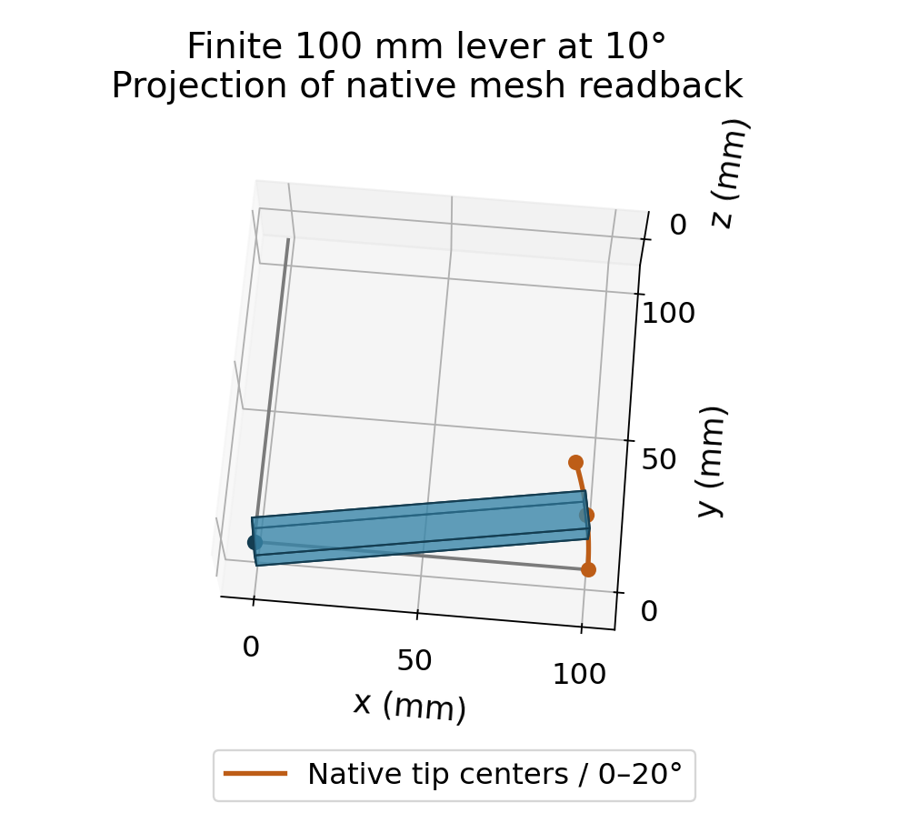
There is also a sampling distinction: the highest angular change divided by time between our selected samples is about 48.495°/s for the short move. The analytic instantaneous peak is 48.990°/s. A finite-interval average should not be relabeled as that peak, even with exact geometry.

Here is the executed standard-library calculation. Zero travel returns a hold; nonpositive model limits are rejected. That rule does not describe the special meaning of zero in any manufacturer’s control table.

from math import sqrt, isclose

def rest_to_rest(distance_deg, speed_cap, acceleration):
    # Positive model limits, not manufacturer register values.
    if distance_deg < 0 or speed_cap <= 0 or acceleration <= 0:
        raise ValueError("Use nonnegative travel and positive model limits")
    if distance_deg == 0:
        return 0.0, 0.0, 0.0
    peak = min(speed_cap, sqrt(acceleration * distance_deg))
    ramp_time = peak / acceleration
    cruise_time = max(0.0, distance_deg / peak - ramp_time)
    return peak, 2 * ramp_time + cruise_time, cruise_time

for travel, cap in [(20, 60), (20, 120), (30, 60), (120, 60)]:
    peak, duration, cruise = rest_to_rest(travel, cap, 120)
    print(f"{travel} deg, cap {cap} deg/s: peak {peak:.3f} deg/s, "
          f"duration {duration:.3f} s, cruise {cruise:.3f} s")

assert rest_to_rest(20, 60, 120) == rest_to_rest(20, 120, 120)
assert isclose(60**2 / 120, 30)  # Travel needed to reach 60 and brake.
assert rest_to_rest(30, 60, 120) == (60, 1.0, 0.0)
assert rest_to_rest(0, 60, 120) == (0.0, 0.0, 0.0)

For an actual position-profile diagnosis, distinguish the configured ceiling, the generated trajectory and the measured motion. An inactive velocity ceiling explains this synthetic short-move result; it does not establish which limit is active on a real machine or whether a higher acceleration is available or appropriate.

Once an input trajectory is defined, the separate slider-crank and Scotch-yoke timing comparison shows why equal input angles and equal output stroke still give different geometric endpoint windows. Its constant-speed input assumption is a separate choice from the rest-to-rest profile used here.