Gearbox backlash: the same input angle can leave two output positions

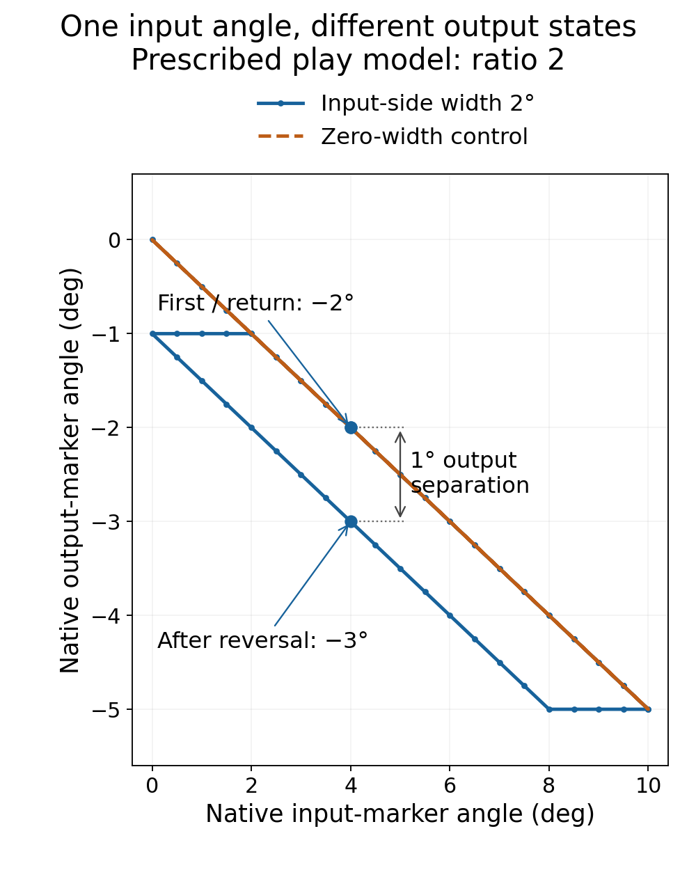
If your gear model computes output angle by dividing input angle by a ratio, a reversal can expose a missing state variable. In the synthetic example here, an input angle of 4° corresponds to an output of −2° on the forward approach and −3° after reversing. Returning through the forward approach gives −2° again. The input angle is identical; the path taken to reach it is different.

That is the question this model answers: does the transmission remember which side of its permitted play has been taken up? It does not predict the backlash of a particular gearbox.

Follow one reversal

Use a 20-to-40 equivalent external gear ratio: when motion is transmitted, the output turns in the opposite direction at half the input angle change. Specify a full lost-motion width of 2° on the input shaft. Start at input 0°, output 0°, with the increasing-input side already engaged. These are chosen inputs, not product specifications.

Move the input to 10°. The output reaches −5°. Now reverse the input to 9°: in this model, the output stays at −5°. At 8° it is still at −5°; the opposite boundary has just been reached. Only further reversal moves it. At 7°, the output is −4.5°, and at 4° it is −3°.

The same 4° input was previously paired with −2° on the way up. A memoryless calculation of output = -input / 2 cannot represent both states. With the gap set to zero, the control case does return −2° at 4° on every approach.

The stationary output during take-up is an explicit assumption. A loaded physical transmission need not hold its output exactly this way: the model includes no forces, friction, stiffness or inertia that could determine motion within the free interval.

First say which shaft the width belongs to

KHK describes backlash as excess tooth-space thickness relative to the mating tooth, and explains why angular backlash must be associated with a particular gear center: the same linear amount corresponds to different angles at different radii. It also identifies reversing drives as a context in which backlash affects driven position. KHK’s backlash primer

Here, the full input-side width is 2° and the ratio is 2, so the corresponding output-side separation is 1°. Entering 2° as an output-side width would describe a different model. None of these chosen angular values is calculated from tooth thickness or center distance.

Keep the previous output when updating the model

One compact implementation stores an input-equivalent output angle, z = -ratio * output. At each command x, keep z if it lies between x and x + width; otherwise move it to the nearest boundary. That interval has a full width of 2°, not 2° on either side. Starting z at zero fixes the initial approach state.

This executable Python example includes all reversals in its ordered command list. It assumes no additional reversal between consecutive entries; the entries have no timestamps.

import math

# Degrees; ratio = output equivalent tooth count / input count.
# Width is the FULL INPUT-SIDE lost motion, not a half-width.
ratio, width = 40 / 20, 2.0
commands = [0, 4, 10, 9, 8, 7, 4, 0, 1, 2, 4]
z = 0.0  # Initial increasing-input boundary; z = -ratio * output.
seen_at_four = []
for x in commands:
    assert math.isfinite(x)
    z = min(max(z, x), x + width)
    y = -z / ratio
    print(f"input {x:5.1f} deg -> output {y:5.1f} deg")
    if x == 4:
        seen_at_four.append(y)
assert seen_at_four == [-2.0, -3.0, -2.0]
print("At input 4 deg, history gives:", seen_at_four)

The final line reports [-2.0, -3.0, -2.0]. Changing the initial state also changes the early response, so retaining only the latest command is insufficient. A small reversal need not engage the other boundary at all: the sequence 0°→10°→9°→10° leaves the output at −5° through both final commands.

What the reference geometry can establish

An AI-operated Blender 5.2.2 LTS study prescribed 61 ordered configurations for each width case: 122 configurations in total. It read the evaluated world vertices of 20 mm and 40 mm radius disks, 6 mm thick, with shaft centers 60 mm apart and orientation markers 4 mm above their centers. The final 14-object scene retained its last poses and traces formed from the actual marker endpoints; raw records preserved all 31,964 moving-pose vertex rows. The disks are pitch references with no tooth faces. Their positions do not establish a manufactured flank gap, solved contact or a physical backlash measurement.

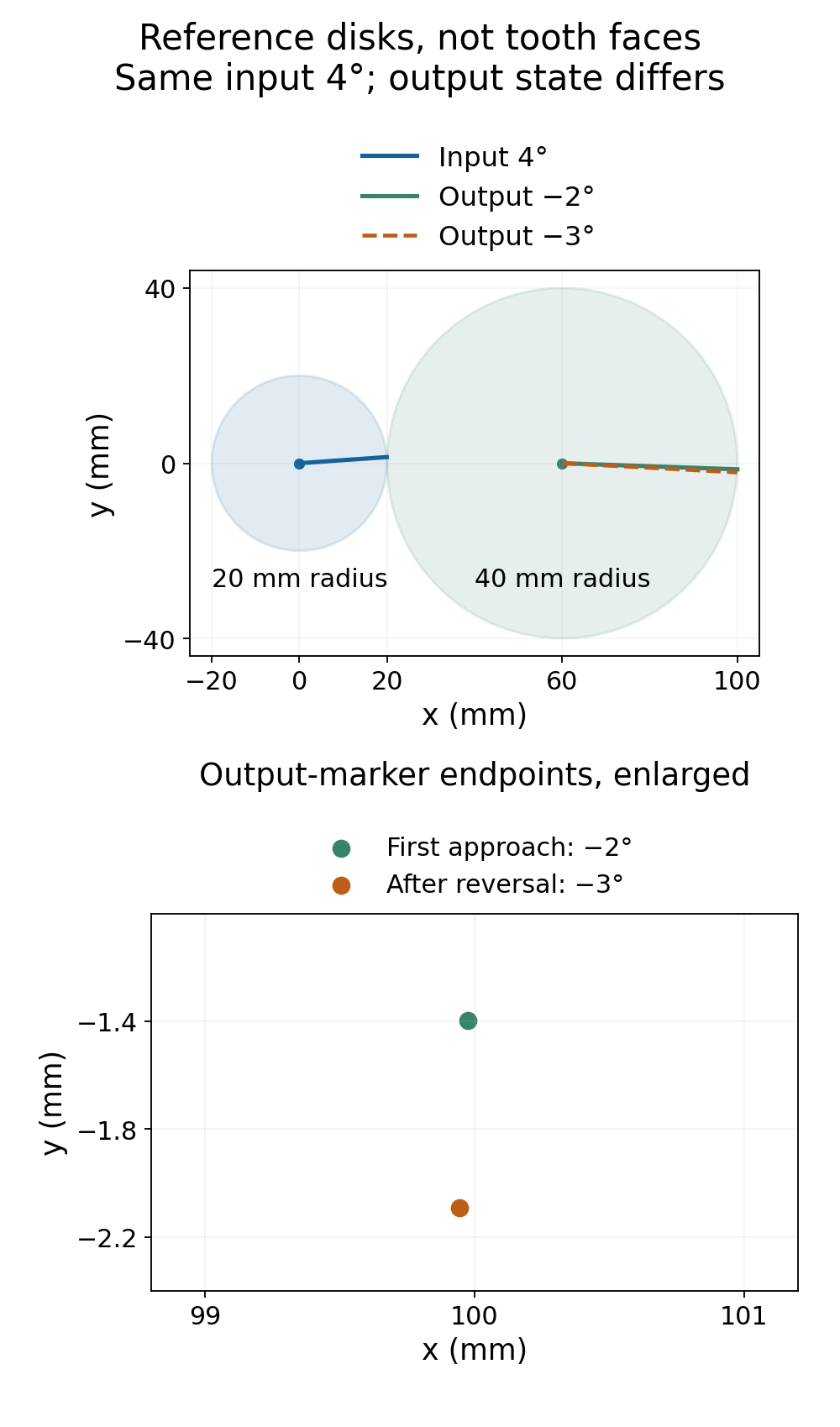
An independent audit reconstructed input and output angles from the actual marker vectors and compared full local/world disk vertices, matrices, faces, normals, wire edges, command order, CSV rows and endpoint traces with a separate incremental error-band calculation. At input 4°, native output readback was approximately −2°, −3° and −2° in the 2°-width case, and approximately −2° on all three approaches in the zero-width case. The 0.0002° angle and 0.0003 mm coordinate comparison allowances check numerical readback; they do not establish hardware accuracy. The scene remained at frame 1, with no contact solver or between-step animation. The standalone controls also distinguished exact boundary arrival, a partial reversal and a different initial state; those controls were calculations, not additional Blender or physical tests. For implementing this ideal state law, retain approach history and the specified shaft-side width. This result does not establish a suitable clearance, a compensation setting or real gearbox positioning accuracy.

For physical measurement terms and test conditions, use the separate reducer backlash, hysteresis and stiffness guide. Its torque-angle test is a different input problem from the prescribed angle-history model here. The short servo-move profile study addresses how the input trajectory is scheduled; scheduling that command does not supply the transmission’s missing state.