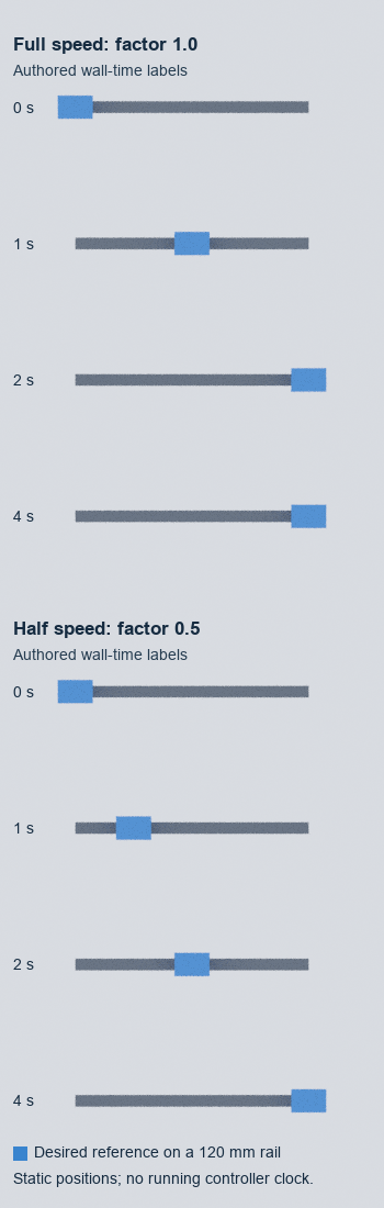
At the same authored wall-time label of 2 seconds, our full-speed reference was at 120 mm while the half-speed reference was at 60 mm. That 60 mm difference was not tracking error. It came from evaluating the same two-second, 120 mm reference with two modeled time progressions: 1.0 × wall label and 0.5 × wall label.
We measured eight finite carriage positions in Blender 5.2.2 LTS. The full-speed row produced 0, 60, 120, and 120 mm at labels 0, 1, 2, and 4 seconds. The half-speed row produced 0, 30, 60, and 120 mm. These were authored static positions, not samples from a running controller or clock.
Equal wall labels produced different reference positions
Both rows used a 120 mm rail and a nominal two-second linear reference. For each row, we recovered the carriage centre from all eight evaluated mesh vertices, reconstructed the rail axis from its finite end faces, and projected the centre onto that axis. The independent audit reproduced all eight declared positions using an authored 8-micrometre comparison allowance for floating-point readback. That allowance describes our numerical check, not measured robot accuracy.
| Authored wall label | Full-speed modeled elapsed | Full-speed position | Half-speed modeled elapsed | Half-speed position |
|---|---|---|---|---|
| 0 s | 0 s | 0 mm | 0 s | 0 mm |
| 1 s | 1 s | 60 mm | 0.5 s | 30 mm |
| 2 s | 2 s | 120 mm | 1 s | 60 mm |
| 4 s | 4 s | 120 mm | 2 s | 120 mm |
The useful debugging observation is the 2-second row: an external monitor following the unscaled schedule expects the endpoint, while the half-speed reference is only halfway along the rail. Calling that difference “60 mm of tracking error” would compare the robot with the wrong desired reference.
For example, a wall-clock-only monitor could pair 2 seconds with 120 mm, subtract a 60 mm position, and report 60 mm of error. A monitor using the authored half-speed reference pairs the same wall label with a 60 mm desired position. Our scene contains no observed robot trace, so it does not claim that either calculation occurred in a controller. It shows why a diagnostic record needs the desired sample that was actually used, rather than reconstructing it later from wall time alone.
Modeled elapsed time and the displayed endpoint are different fields
We kept modeled virtual elapsed time unclamped: factor × wall label. We separately displayed a finite two-second reference using min(2 s, modeled elapsed). That distinction is clearest at the 4-second label.
For the full-speed row, modeled elapsed time was 4 seconds, while the displayed reference time had reached its two-second endpoint and the carriage remained at 120 mm. For the half-speed row, modeled elapsed time was 2 seconds and the carriage had just reached the same 120 mm endpoint. The endpoint clamp belongs to our finite display model. It is not a claim that the controller cursor itself clamps at the final trajectory time.
The two 120 mm boxes at the final label therefore look identical while carrying different modeled elapsed values. Geometry alone cannot recover that distinction. A useful visualization or log must retain the time-base fields instead of assuming that equal positions imply equal progress histories.
This distinction prevents two common logging mistakes. First, do not overwrite virtual elapsed time with a clamped path coordinate; retain both. Second, do not infer a controller clock from a Blender label. Our labels supplied the arithmetic inputs, but Blender did not measure elapsed execution time.
What the examined controller sources add
The official speed-scaling documentation distinguishes on-robot and on-controller scaling. With on-robot scaling, hardware reports a scaling value and performs the reduced motion. With on-controller scaling, the controller generates reduced commands while the hardware is unaware of scaling; the examined implementation notes that this mode currently works with position-based interfaces.
The pinned controller source shows that the trajectory cursor advances by controller period times the scaling factor. A subtle but important detail is that next-command sampling adds the full update period. The simple equation in our static scene illustrates reference progression; it does not reproduce every controller sampling step.
The same pinned documentation says that path error is compared with the scaled trajectory and goal-time tolerance uses virtual trajectory time. If an application must enforce the original wall-clock schedule, it needs external monitoring. This time-base issue is separate from the path-versus-goal position checks in our preceding experiment.
Log the time base before diagnosing lateness
A useful trace should make these fields explicit:
- Record the scaling mode and current factor rather than only the commanded position.
- Log wall time and the controller’s trajectory cursor as separate values.
- Log the desired state sampled from that cursor alongside observed state.
- Identify whether a monitor uses virtual goal time or an external wall-clock deadline.
- Keep controller period and next-command sampling visible when one-cycle differences matter.
This also differs from policy frequency versus controller calls. That article asks how often a goal changes and how often a controller computes output. Here, the reader question is how far the desired trajectory reference should have advanced under a scaling factor.
Our experiment verified static finite geometry and the arithmetic that placed it. It did not execute ROS 2, ros2_control, Joint Trajectory Controller, a speed-scaling interface, interpolation, tracking tolerances, an action result, a deadline, robot dynamics, or hardware. The 1.0 and 0.5 factors, two-second duration, and 120 mm rail are explanatory inputs rather than recommended settings. The conclusion is narrow and practical: before calling a scaled trajectory late, check which clock produced the reference you are comparing against.