A scan contains measurements taken at different times. If the sensor moves while collecting them, putting every return at the initial sensor pose can make a straight wall appear curved. The ranges can be correct; their placement can still be wrong.
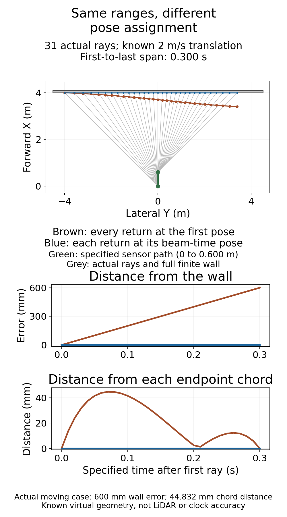
In our controlled virtual example, a sensor moves a specified 0.600 m toward a stationary wall over the 0.300 s between the first and last rays. Reconstructing all 31 returns at its first pose leaves points as much as 0.600 m away from the wall. They are also noncollinear: their largest distance from the line through the first and last reconstructed points is about 44.8 mm. Using each beam’s specified pose places the same ranges back on the wall within numerical rounding.
The header is the beginning of this scan
The official ROS Rolling LaserScan definition, checked on October 6, 2026, says its header timestamp is the acquisition time of the first ray. time_increment is the time between measurements, while scan_time is the time between scans. It also defines angles about positive Z, with zero along forward X, and ranges in metres. These fields describe the message convention; they do not verify a device’s timestamps. ROS: LaserScan definition
Our first stamp is 12.500 s and the interval is 0.010 s. For index i, the specified time is 12.500 + i * 0.010. With 31 rays, the final index is 30 and the last stamp is 12.800 s. There are 30 intervals between the first and last samples.
We deliberately set the separate inter-scan scan_time to 0.400 s. Dividing that value across the rays would give a different timing model. All of these numbers are chosen study inputs, not specifications of a scanner.
Keep the range; change the pose assigned to it
The wall’s front face is at X=4 m, extends from Y=−4.5 to +4.5 m, and has a 1 m height and 0.1 m thickness. The horizontal fan runs from −45° to +45° inclusive in 3° steps. The first sensor pose is the identity at the origin. The moving case translates along +X at a known 2 m/s without rotating; the stationary control uses zero velocity.
For a return with range r and unit direction d, the incorrect reconstruction is O_first + r*d. The compensated reconstruction is O_beam + r*d, where O_beam is the origin at that ray’s specified time. The range and angular direction are identical in both calculations.
This also separates two meanings of using the first frame. Correct deskew can express every point in the first reference frame after applying the relative beam-time pose. Assigning the first pose to every return skips that correction. Our first frame is identity, so the corrected first-frame coordinates equal the world coordinates.
The reader example calculates the ideal front-wall intersection directly. Every ray is checked against the finite wall width and the chosen 0.05–8 m range interval.
import math

count, dt, first_stamp = 31, 0.010, 12.5
wall_x = 4.0  # metres; finite wall front has -4.5 <= y <= 4.5

def chord_error(points):
    x0, y0 = points[0]
    dx, dy = points[-1][0] - x0, points[-1][1] - y0
    return max(abs(dx*(y-y0) - dy*(x-x0)) / math.hypot(dx, dy)
               for x, y in points)

for velocity in (0.0, 2.0):  # prescribed m/s toward the wall, no rotation
    first_pose, beam_pose = [], []
    for i in range(count):
        elapsed = i * dt
        angle = math.radians(-45 + 90 * i / (count - 1))
        direction = (math.cos(angle), math.sin(angle))
        origin_x = velocity * elapsed
        distance = (wall_x - origin_x) / direction[0]
        local_point = [distance * component for component in direction]
        correct = (origin_x + local_point[0], local_point[1])
        assert 0.05 <= distance <= 8 and -4.5 <= correct[1] <= 4.5
        first_pose.append(local_point)  # first pose is identity at (0, 0)
        beam_pose.append(correct)       # same range, now use this beam's pose
    assert max(abs(x-wall_x) for x, y in beam_pose) < 1e-12
    wall_error = max(abs(x-wall_x) for x, y in first_pose)
    print(f"v={velocity:.1f} m/s: wall error={wall_error:.3f} m; "
          f"endpoint-chord deviation={1000*chord_error(first_pose):.3f} mm")
print(f"First/last stamps: {first_stamp:.3f}, "
      f"{first_stamp+(count-1)*dt:.3f} s; span={(count-1)*dt:.3f} s")
The stationary row reports zero wall error and zero chord deviation to the printed precision. The moving row reports 0.600 m and 44.833 mm. The chord measure establishes that the naïve points do not merely form another displaced straight line; it is not a fitted-wall residual or a sensor-accuracy metric.
What this comparison can establish
An AI-operated Blender 5.2.2 LTS experiment on October 6, 2026 made 62 actual Scene.ray_cast calls: 31 stationary and 31 moving. A single closed wall mesh was present during the queries. The scene later contained nine objects and 318 evaluated vertices, including edge-only drawings of the rays, sensor paths and both point reconstructions. Those display drawings were added after the queries and did not serve as hit targets.
The Blender API documents evaluated world-space ray geometry. We preserved the actual float origins and normalized direction arguments, returned world hits, face indices, normals and hit-object matrices. Every query hit the finite front wall within the declared 0.05–8 m interval. Each range was computed as the distance from the passed origin to the returned hit; the API did not return a separate LiDAR range measurement. Calls ran at static scene frame 1. The specified beam timestamps are synthetic study inputs, not wall-clock measurements of Blender execution.
A separate audit computed finite-box intersections by a slab method, derived origins from each specified acquisition timestamp, and checked every actual range and reconstructed point, all mesh vertices/topology, 62 CSV rows, append-only query records, scene export and source hashes. Original authored and evaluated scenes, context and the base file were unchanged.
In the actual moving readback, maximum first-pose wall error was 0.599999607 m and endpoint-chord distance was 44.832206 mm. Beam-time wall error stayed below 0.0005 mm and chord distance below 0.001 mm. The ideal standalone reader reports 44.833 mm after rounding; its small difference from the actual 44.832 mm output is floating-point geometry, not sensor noise. The independent geometry checks allowed 0.01 mm; passed origins used 0.001 mm and direction arguments used a dimensionless tolerance of 0.0000003. These are consistency allowances, not hardware accuracy. Standalone controls rejected 22 deliberate corruptions and five invalid inputs, including wrong timing, pose, face, units and fabricated reconstruction.
The result is specific to the stated motion and scene. A separate calculation with translation parallel to the wall leaves the naïve points collinear even though their individual positions are wrong. A straight-looking wall alone therefore cannot validate timing or motion compensation.
For this reconstruction, the useful missing association is range → acquisition time → sensor pose. The example assumes those times and poses are known. It neither estimates missing motion nor demonstrates a driver’s timestamps, clock synchronization, SLAM trajectory or a deskew product’s performance.
If you are choosing the sensor and scan representation, the existing 2D versus 3D LiDAR guide supplies that broader context. This experiment isolates the next coordinate question: associate each usable return with its acquisition time and the pose at that time before comparing its position with the map. It assumes a static scene, known poses and no rotation; moving objects, estimated trajectories, synchronization uncertainty and rotating extrinsics require further checks.