In robosuite’s Controller.scale_action, check the current input clipping bounds together with the cached action_scale, action_input_transform and action_output_transform actually in use. An input at the centre of the allowed range maps to the output midpoint only when those affine coefficients match the stated bounds. Zero input is therefore not automatically a neutral command, and changing bound fields after initialization can leave the cached map unchanged. Different raw commands can also become identical after clipping. Check both clipping and the active map before interpreting an unexpected positional delta as a gain or tracking problem.
Consider a controller log in which (0, 0, 0) seems to request a positive x increment, while increasing x from 1 to 2 changes nothing. Both observations can follow directly from the configured action map. Neither observation, by itself, identifies what the robot moved or what its actuators received.
The source reading below is pinned to robosuite v1.5.2, commit 824ac14cefcfb7ec125fe5eb2e0bad7364466154, checked October 6, 2026. The numerical examples are authored predictions for a fixed-impedance, three-dimensional positional delta. They are not robosuite execution results. A separate Blender experiment measures static geometry constructed from those authored predictions. It tests the finite marker coordinates, not robosuite controller behaviour.
Which part of the action is being scaled?
Start with the spatial command that actually reaches the controller. A whole robot action vector may also contain other part commands or impedance parameters. Feeding that entire vector into a three-component calculation would answer the wrong question even if the arithmetic were correct.
The pinned OSC dimension and bounds setup selects three spatial components for position control and six when orientation is included. Its goal-setting branch then separates impedance fields before scaling the remaining goal update. Fixed impedance uses the supplied action as that update; variable impedance and variable stiffness remove their leading parameter fields first.
For this example, that separation leaves exactly (a_x, a_y, a_z). The values are dimensionless inputs. Their output bounds are authored in metres, so the result represents a positional increment. Orientation components, stiffness parameters, and actuator commands do not share that unit contract. If the command appears to affect the wrong robot part, resolve the composite action-vector slice before examining scaling.
How do clipping and the midpoint produce the result?
The base controller’s scaling helper applies an affine map independently to each component. For one axis with valid ordered bounds, its calculation can be written as:
clipped = clip(raw, input_min, input_max)
scale = abs(output_max - output_min) / abs(input_max - input_min)
scaled = (clipped - input_midpoint) * scale + output_midpoint
Each midpoint is the average of its minimum and maximum. Subtracting the input midpoint recentres the clipped value; adding the output midpoint places it in the configured output interval. The absolute values reproduce this pinned implementation’s width calculation. They do not establish useful behaviour for reversed or zero-width bounds.
Use the following two authored configurations to isolate the midpoint. Only the x output interval changes; its width remains 0.08 m. The y and z settings stay identical. These are deliberately chosen examples, not documented defaults or tuning recommendations.
| Axis | Dimensionless input interval | Symmetric output interval, m | Asymmetric-x output interval, m |
|---|---|---|---|
| x | [-1, 1] |
[-0.04, 0.04] |
[-0.02, 0.06] |
| y | [-1, 1] |
[-0.04, 0.04] |
[-0.04, 0.04] |
| z | [-1, 1] |
[-0.01, 0.01] |
[-0.01, 0.01] |
Both cases have x scale 0.04 m per input unit. The symmetric x midpoint is zero; the asymmetric midpoint is 0.02 m. Consequently, before considering any target reference, the authored x formulas are 0.04 * clipped_x and 0.04 * clipped_x + 0.02.
Why does zero input differ from zero increment?
For the asymmetric configuration, raw x equal to zero is already the input midpoint. It therefore maps to 0.02 m. To obtain zero scaled x, solve 0.04 * a_x + 0.02 = 0, giving a_x = -0.5. This value is inside the input interval, so clipping does not alter it.
Here are three authored predictions using full three-component commands. Every output tuple is in metres; the input tuples are dimensionless.
| Supplied command | Symmetric predicted increment, m | Asymmetric-x predicted increment, m |
|---|---|---|
(0, 0, 0) |
(0, 0, 0) |
(0.02, 0, 0) |
(-0.5, 0, 0) |
(-0.02, 0, 0) |
(0, 0, 0) |
(0.5, 0.5, 0) |
(0.02, 0.02, 0) |
(0.04, 0.02, 0) |
The second row is a useful diagnostic counterexample: the same negative input that cancels the asymmetric midpoint requests a negative increment in the symmetric case. A neutral input is configuration-dependent. Copying -0.5 into another controller configuration would not preserve its meaning.
For another valid interval, solve the same equation using its own coefficients: neutral_input = input_midpoint - output_midpoint / scale. Then check whether that value lies inside the allowed input interval. If zero lies outside the output interval, no in-range input can produce zero through this map. Increasing the magnitude of an out-of-range input cannot reach it either, because clipping happens first. This is a property of the chosen mapping, so record it before trying to compensate with a command from a different configuration.
Keep three observations separate in a log: the supplied input, the scaled increment, and the eventual controller output. A zero increment does not establish zero actuator assignment. It does not even identify the positional target until the reference used to construct that target is known. The achieved-position versus previous-goal delta explanation starts at that next boundary, after the delta already has positional units.
Why can x commands of one and two have the same effect?
With input bounds [-1, 1], the helper clips raw x equal to 2 down to 1 before applying either output map. The y component 0.5 remains unchanged. Thus (1, 0.5, 0) and (2, 0.5, 0) have the same predicted scaled increment within each configuration.
The table keeps both inputs visible. Its output columns show only x and y; z remains zero in every row. These are arithmetic predictions, not observed motion.
| Raw command | Clipped command | Symmetric output (x, y), m |
Asymmetric-x output (x, y), m |
Reason |
|---|---|---|---|---|
(1, 0.5, 0) |
(1, 0.5, 0) |
(0.04, 0.02) |
(0.06, 0.02) |
x is on its bound |
(2, 0.5, 0) |
(1, 0.5, 0) |
(0.04, 0.02) |
(0.06, 0.02) |
Excess positive x is clipped |
(-2, -0.5, 0) |
(-1, -0.5, 0) |
(-0.04, -0.02) |
(-0.02, -0.02) |
Excess negative x is clipped |
If only the scaled result is recorded, the first two rows become indistinguishable. Preserve the raw command alongside it when investigating saturation. Equal scaled values establish equality at this mapping boundary; different controller state, target history, or later processing could still produce different downstream results.
The equality is not unique to those two examples. Holding y and z fixed, every raw x at or above 1 maps to the positive x endpoint under these bounds. A sequence of increasingly large raw values can therefore hide a persistent saturation problem behind an unchanged scaled log. Compare how often the raw value exceeds its bound, rather than inferring that the upstream policy issued an unchanged command.
Does action scaling preserve a vector’s direction?
Componentwise clipping does not divide a vector by its length. For the raw command (2, 0.5, 0), the y-to-x ratio is 0.25; after clipping it becomes 0.5. A vector-length normalization would preserve that ratio. This distinction explains why a larger raw x command can change the intended direction while leaving the clipped result unchanged.
The affine map can also change direction relative to the fixed origin without clipping. The in-range command (0.5, 0.5, 0) has equal x and y. Our symmetric map preserves that equality in the x-y plane, while the asymmetric map produces (0.04, 0.02, 0). The added x midpoint changes the ratio. Unequal per-axis scale factors can introduce another change; neither operation is a unit-vector normalization.
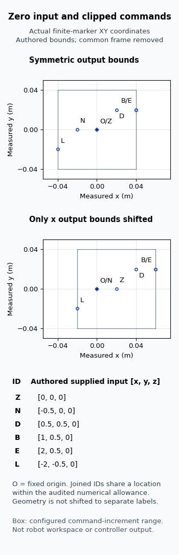
The experiment created two static scenes with 16 separate closed rectangular meshes: one range box, one fixed-origin marker and six command markers per case. Each mesh has eight corners; the independent check used all 128 actual Blender corner coordinates to recover marker centres and each range box. A declared common rigid transform was removed before comparing those coordinates in metres. No geometry was shifted to make coincident commands appear separate.
In the asymmetric case, the measured zero-input marker was approximately 0.020000010 m along x from the fixed-origin marker, with y and z differences below 5e-9 m. The (-0.5, 0, 0) marker coincided with that origin. The two positive commands (1, 0.5, 0) and (2, 0.5, 0) had identical measured centres within each case: approximately (0.0400000, 0.0200000, 0) m relative to the origin in the symmetric case, and (0.0600000, 0.0200000, 0) m in the asymmetric case. These agree with the authored calculations within the fixed 8e-6 m derived-distance allowance; the extra displayed digits describe mesh-coordinate arithmetic, not robot measurement precision.
The figure uses separate finite markers, including separate markers for commands that coincide after clipping. Read the marker centres against the output intervals. A marker has a visible width for readability, so its outer faces are not a test of whether the whole marker fits inside the interval box. These static coordinates also provide no evidence about collision, reachability, controller accuracy, or physical safety.
What should be checked before changing the bounds?
Record the actual per-axis arrays, not just a configuration label such as “normalized action.” The pinned scalar-to-array helper broadcasts a scalar to the requested dimension and converts an iterable into an array. That conversion alone is not a general guarantee of matching length, finite numeric values, or correctly ordered bounds.
For a reproduction of this example, require three finite numeric components and three matching bounds per side, with minimum strictly below maximum on every axis. Reject malformed inputs explicitly rather than treating an exception, a nonfinite value, or accidental broadcasting as a meaningful scaled command. The arithmetic here assumes positive input and output widths throughout.
There is also an initialization detail: scale_action computes its scale and both midpoint transforms only when action_scale is None. Later calls use those cached quantities. Editing bound fields after that first calculation does not make the displayed helper automatically rebuild its affine coefficients. Its clipping call still reads the input bounds, which makes a partial configuration change especially easy to misinterpret. Compare the current bounds with the coefficients actually in use and the supported controller initialization path before drawing conclusions from a changed configuration.
Finally, confirm input_type. In the shown OSC delta branch, the spatial update passes through scale_action; in the absolute branch, the first three goal-update components are assigned directly to goal_pos. Applying this scaling explanation to that absolute branch would insert an operation absent from the cited code. This is a statement about the inspected branch, not every controller or every later processing stage.
Which log entry will locate the mismatch?
Capture one command’s path in order: the named part’s action slice, the impedance-parsed spatial update, the input bounds, the clipped components, the cached affine coefficients, and the scaled result. Keep the raw and clipped values in dimensionless units and the positional result in metres. A discrepancy before the scaled result points to parsing, bounds, clipping, or the map itself; a discrepancy after it requires a separate investigation of the target reference and downstream controller behaviour.
If the uncertainty concerns how often goals or controller calls happen, use the control-frequency and goal-update explanation. If it concerns converting an action schema between robot embodiments, the broader action-normalization guide covers that different mapping problem.
For this specific diagnosis, retain the input that disappeared through clipping and the midpoint that shifted zero. Those two values explain the authored examples without inferring motion from a command. Actual robosuite, MuJoCo, controller, actuator, and hardware execution have not been performed here.