Two path segments can meet at exactly the same point and still demand a change in direction, speed or acceleration at the join. The useful question is what must remain continuous for the intended motion, and whether the time assigned to each segment preserves that continuity.
In five Blender examples, every pair has the same boundary point. We progressively match tangent direction, first derivatives and second derivatives, then change the duration of the outgoing segment. Geometry and timing impose separate conditions: the same shape can still produce a speed or acceleration jump.
We generated the curve samples and control markers in Blender 5.2.2 LTS on 6 October 2026, then read their saved three-dimensional coordinates. An independent calculation reconstructed the marker centers, compared the samples with the cubic formula and checked the endpoint derivatives. The plot projects those saved coordinates into their local frame. Rates come from supplied timing, not from a running robot. This is an AI-operated numerical study.
A smooth-looking tangent can still hide a speed change
Write the left segment’s controls as P0 through P3 and the right segment’s controls as Q0 through Q3. Each segment uses its own parameter u from 0 to 1. Setting P3 equal to Q0 closes the positional gap, called C0 continuity. It says nothing about the direction in which the path approaches or leaves that point.
At the join, the incoming segment’s ending derivative is 3(P3 − P2) and the outgoing segment’s starting derivative is 3(Q1 − Q0). If these nonzero vectors point in the same direction, the join has regular G1 continuity. Oppositely directed vectors do not qualify, and a zero derivative does not provide a defined tangent direction for this test.
The two vectors must also have equal magnitude to match the first derivatives in the declared u parameters, a C1 join. A collinear pair with one vector half as long gives the same tangent direction but a different rate of progress if both segments receive the same duration. A drawing of the curve alone can make that difference easy to miss.
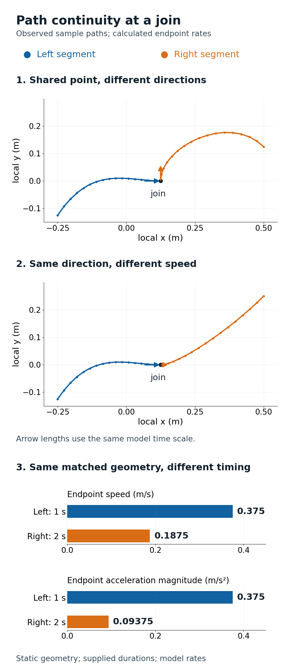
Our left segment ends at (0.125, 0, 0) m, with first derivative (0.375, 0, 0) m per unit u. In the parallel-tangent alternative, the right starting derivative is (0.1875, 0, 0). Both segments take one supplied second. The direction matches, but the starting speed on the right is half the ending speed on the left. The corner alternative changes the right derivative to (0, 0.375, 0), so even its direction fails to match.
Matching velocity leaves another boundary condition
Moving Q1 to make the first derivatives equal fixes that velocity mismatch for equal durations. It does not automatically match the second derivatives. Those are 6(P3 − 2P2 + P1) on the left and 6(Q2 − 2Q1 + Q0) on the right.
The left second derivative in this example is (0, 0.375, 0) m per unit u squared. The matched-velocity alternative has a right second derivative of (0, 0.75, 0). With one second on each side, the velocity is continuous but acceleration changes at the boundary. A further adjustment of Q2 makes both second derivatives (0, 0.375, 0), giving a C2 join in the specified segment parameters.
These are endpoint conditions, not statements about constant speed or acceleration along either segment. They also do not check jerk, actuator limits, robot inverse kinematics, collision clearance or dynamic tracking. Here the curves describe a Cartesian reference point; they are not a validated robot joint trajectory.
Keep the time conversion attached to the curve
For a segment assigned duration T with u increasing linearly in elapsed time, velocity = dB/du / T and acceleration = d²B/du² / T². This chain rule is part of the model. It would change for a different, nonlinear time law.
The final alternative uses exactly the same right-hand controls as the C2 geometry but gives that segment two seconds instead of one. Its starting velocity becomes (0.1875, 0, 0) m/s and its starting acceleration becomes (0, 0.09375, 0) m/s². The left values remain (0.375, 0, 0) m/s and (0, 0.375, 0) m/s². The geometric join has not changed, yet neither time-scaled derivative matches.
Conversely, unequal u derivatives can sometimes be made to match in time by choosing different durations. That does not guarantee acceleration continuity too, because acceleration depends on the square of duration and on a different combination of control points. Keep the position, tangent direction, first derivative, second derivative and time-scaled results separate instead of giving the entire join one undifferentiated smooth label.
The ROS 2 Control Jazzy trajectory documentation makes a related interface distinction: the spline strategy depends on which waypoint fields are supplied. It describes position-level continuity for position-only linear interpolation, velocity-level continuity when cubic interpolation uses position and velocity, and acceleration-level continuity when quintic interpolation uses position, velocity and acceleration.
Those guarantees belong to the documented interpolation and waypoint constraints. Arbitrary cubic segments do not automatically share velocity. Our deliberately chosen Bézier controls are an independent geometric example, not an execution of that controller or a claim that its implementation uses this representation. A specially matched pair of cubics can have a C2 boundary without implying that arbitrary position, velocity and acceleration constraints can always be satisfied by a cubic segment.
The five comparisons produced this pattern. The incoming segment takes one second in every case. The outgoing duration is shown separately. Continuity requires matching vectors, not merely matching their magnitudes.
| Join arrangement | Outgoing duration | Velocity continuous | Acceleration continuous |
|---|---|---|---|
| Corner | 1 s | No | No |
| Parallel tangents | 1 s | No | No |
| Matched first derivatives | 1 s | Yes | No |
| Matched first and second derivatives | 1 s | Yes | Yes |
| Same matched geometry, longer duration | 2 s | No | No |
Stored-coordinate checks allowed 4 µm per component. Derived velocities and accelerations used comparison bounds of 0.0001 m/s and 0.0005 m/s². These allowances handle numerical representation; they are not robot tracking tolerances.
The Bézier spacing study explains why equal changes in u do not imply equal travel distances. Sample spacing within a curve and the two derivatives meeting at a join require different checks.
Calculate the join from the controls, not adjacent sample spacing
This short standard-library source contains the exact five local-frame inputs and supplied durations. It computes endpoint derivatives directly and prints the magnitudes of their jumps. It uses elementary arithmetic, with no Blender, ROS interpolation or robot-interface calls.
import math

def endpoint(control, at_end, duration):
    if duration <= 0 or not math.isfinite(duration):
        raise ValueError('Duration must be positive and finite')
    p = control
    if at_end:
        first = [3*(p[3][j]-p[2][j]) for j in range(3)]
        second = [6*(p[3][j]-2*p[2][j]+p[1][j]) for j in range(3)]
    else:
        first = [3*(p[1][j]-p[0][j]) for j in range(3)]
        second = [6*(p[2][j]-2*p[1][j]+p[0][j]) for j in range(3)]
    return [v/duration for v in first], [a/duration**2 for a in second]

def jump(a, b):
    return math.sqrt(sum((x-y)**2 for x, y in zip(a, b)))

left = [(-.25, -.125, 0), (-.125, .0625, 0), (0, 0, 0), (.125, 0, 0)]
right = [
    ('corner', (.125, .125, 0), (.375, .25, 0), (.5, .125, 0), 1),
    ('parallel tangent', (.1875, 0, 0), (.375, .125, 0), (.5, .25, 0), 1),
    ('matched velocity', (.25, 0, 0), (.375, .125, 0), (.5, .25, 0), 1),
    ('matched acceleration', (.25, 0, 0), (.375, .0625, 0), (.5, .25, 0), 1),
    ('duration change', (.25, 0, 0), (.375, .0625, 0), (.5, .25, 0), 2),
]
v_left, a_left = endpoint(left, True, 1)
for name, p1, p2, p3, seconds in right:
    control = [left[-1], p1, p2, p3]
    v_right, a_right = endpoint(control, False, seconds)
    print(f'{name}: velocity jump={jump(v_left, v_right):.6f} m/s, '
          f'acceleration jump={jump(a_left, a_right):.6f} m/s^2')
A single rotated and translated frame was applied to every alternative. Control and curve-sample positions were recovered from the centers of finite markers and checked against independently evaluated cubic positions. Endpoint derivatives came from the recovered control centers. A last-sample chord divided by its interval is an average displacement rate; it cannot replace the endpoint derivative.
The arrangements are static alternatives in a common frame. The plotted sample lines have no physical thickness; supplied durations do not cause playback or measure velocity. The native samples, stored geometry and derived endpoint vectors passed the fixed numerical comparisons. We did not run ROS, Mimic, a learned policy, a controller, a physics solver or hardware. Before using a join in a motion system, establish its required continuity and actual timing contract, then check joint limits, collisions and tracking.