The average of left and right wheel travel gives the signed path length of the axle midpoint in an ideal differential-drive model. It is not automatically a straight displacement in the starting direction, and it is not a world-X increment. When the wheels travel different distances, the heading changes during the update. Keeping that finite turn changes the predicted endpoint.
This is an AI-operated, synthetic geometry study completed in Blender 5.2.2 LTS on October 5, 2026. Four conditions used 68 prescribed static body/wheel poses, followed by a separate circle-geometry audit of the evaluated mesh vertices and virtual wheel markers. There was no wheel-ground rolling, slip, physical encoder, controller, ROS or hardware test.
A 250 mm average does not mean 250 mm straight ahead
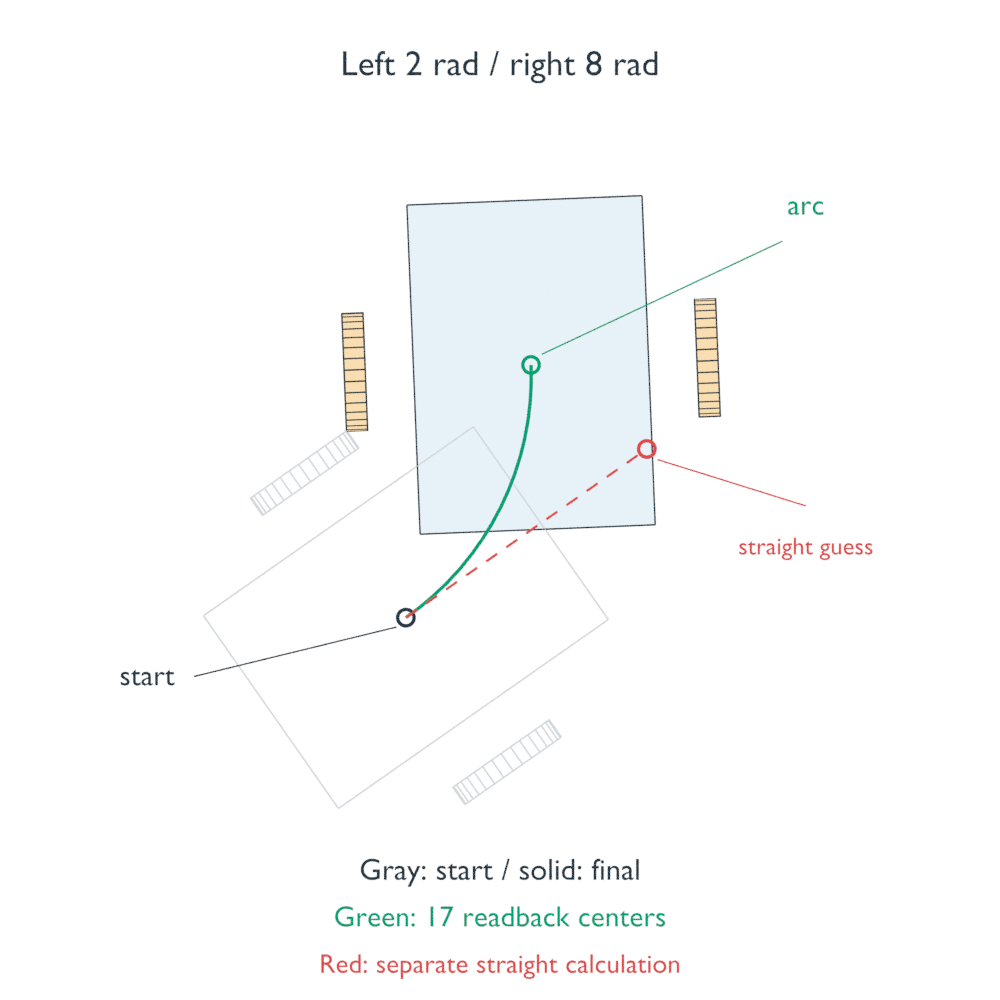
Take two nominal 50 mm radius wheels with 300 mm between their rolling-path centerlines. Start the axle midpoint at (400, −200) mm with the body’s forward direction 35° from world X. Define positive wheel rotation as forward travel on both sides.
For left/right increments of 2 and 8 rad, the ideal wheel travel values are 100 and 400 mm. Their average is 250 mm, and their difference divided by the 300 mm track gives a 1 rad heading change. This example prescribes a constant left/right increment ratio throughout the interval, so the axle midpoint follows a constant-curvature arc.
Its calculated endpoint is (506.405, 14.803) mm, with heading 92.295780°. Taking the 250 mm average along only the starting heading misses that endpoint by 121.566 mm. Even if the arc displacement is calculated correctly in the body frame, adding its components directly to world X/Y without the starting 35° rotation misses by 144.166 mm.
Those differences are errors between mathematical constructions under the same synthetic inputs. They are not measured odometry drift or controller performance.
The ROS 2 control mobile-robot kinematics documentation separates body forward motion from yaw using the average and difference of wheel speeds. Its unicycle equations also rotate body-forward motion into world coordinates using the heading. The finite-interval calculation here integrates that ideal geometry rather than treating the initial heading as constant during a turn.
The straight and spinning cases belong in the same calculation
Let the wheel travel increments be dL and dR, their average be s, and the turn be a:
dL = r·deltaPhiL; dR = r·deltaPhiR; s = (dL+dR)/2; a = (dR−dL)/track
For a constant-curvature interval, the signed chord length is s·sinc(a/2), where sinc(z) = sin(z)/z and sinc(0) = 1. The chord points along the starting heading plus half the turn. Add that chord in world coordinates, then add a to the heading.
This also covers two useful boundary cases. Equal 4 rad increments produce a 200 mm straight movement along the initial 35° heading. Opposite increments of −3 and +3 rad rotate the body by 1 rad while leaving the axle midpoint at its starting XY position. Other points on the finite body still change position during that rotation.
For a near-straight pair of 4 and 4.0006 rad, the turn is only 0.0001 rad. A stable sinc evaluation approaches the straight result continuously. The code below uses a short series near zero, avoiding division by zero and unnecessary cancellation. All angles inside the update are radians; the heading is converted to degrees only for printing.
from math import sin, cos, radians, degrees, hypot

radius, track = .05, .30   # meters
start = (.4, -.2, radians(35))

def update(left_rad, right_rad, pose=start):
    left, right = radius*left_rad, radius*right_rad
    distance = (left+right)/2
    turn = (right-left)/track
    half = turn/2
    sinc = 1-half*half/6+half**4/120 if abs(half) < 1e-4 else sin(half)/half
    chord = distance*sinc
    x, y, heading = pose
    return (x+chord*cos(heading+half), y+chord*sin(heading+half), heading+turn)

for name, left, right in [('straight', 4, 4), ('in place', -3, 3),
                          ('arc', 2, 8), ('small angle', 4, 4.0006)]:
    x, y, heading = update(left, right)
    print(f'{name}: x={x*1000:.3f} mm, y={y*1000:.3f} mm, '
          f'heading={degrees(heading):.6f} deg')

exact = update(2, 8)
straight_guess = (start[0]+.25*cos(start[2]), start[1]+.25*sin(start[2]))
print(f'Arc versus initial-heading straight guess: '
      f'{hypot(exact[0]-straight_guess[0], exact[1]-straight_guess[1])*1000:.3f} mm')
assert hypot(update(-3, 3)[0]-start[0], update(-3, 3)[1]-start[1]) < 1e-12
subdivided = start
for _ in range(8):
    subdivided = update(2/8, 8/8, subdivided)
assert max(abs(a-b) for a, b in zip(subdivided, exact)) < 1e-12
Splitting the arc into eight proportional subincrements gives the same endpoint. Changing the order is a different assumption: applying all the left increment and then all the right increment leaves the same wheel totals but a calculated endpoint 64.034 mm from the constant-curvature result. Two total wheel readings do not reveal an arbitrary path between them.
What the mesh readback verifies, and where it stops
The native study used a 280 × 200 × 50 mm chassis and two 32-sided wheel meshes, each 18 mm wide. Seventeen prescribed samples per condition retained every evaluated vertex and face, the body position, wheel centers and a virtual spoke on each wheel. An independent audit recovered heading from the finite chassis and wheel angles from those markers, then reconstructed the pose with circle geometry rather than calling the producer’s chord helper.
All four conditions agreed within the numerical comparison limits: 5 micrometers for finite vertices and 20 microradians for angles. These are audit tolerances, not measured hardware accuracy. The native arc endpoint rounded to (506.405, 14.803) mm; the straight endpoint rounded to (563.830, −85.285) mm. The in-place midpoint rounded to (400.000, −200.000) mm, with tiny floating-point readback differences. The near-straight endpoint rounded to (563.837, −85.268) mm.
The samples matter for the 8 rad wheel increment: a final spoke position alone contains only a wrapped angle. Sequential marker changes smaller than π retain the chosen winding count. This is virtual geometry readback, not an encoder experiment. The polygonal wheel mesh is also not being rolled across a simulated ground plane.
The diff_drive_controller documentation identifies wheel radius, separation and feedback interfaces, including an open-loop option. That is controller context, not a configuration tested here. The captured odometry implementation also has small-angle branches: the current integrate() and deprecated integrateExact() do not use identical approximations. This reader calculation is an ideal constant-curvature check, not a bit-for-bit reproduction of either method. The referenced Rolling documentation is for a development version.
For an implementation check, preserve the left/right convention and units, rotate the displacement using the starting body heading, and make the within-interval motion assumption explicit. If an otherwise consistent estimate drifts on a physical robot, the next question is different: the wheel odometry slip and covariance guide covers calibration, traction and uncertainty. This mesh readback establishes consistency of the prescribed finite geometry; it cannot establish real wheel radius, ground traction, slip, encoder accuracy or localization performance.