Two IMUs with parallel axes on the same rotating body need not have the same acceleration. A sensor at the rotation center can remain in place while a sensor farther out travels around it. Rotating both vectors into the same axes does not remove that difference: they describe different points. Before comparing an IMU signal with acceleration assigned to a robot’s body origin, check where that origin and the sensor are located.
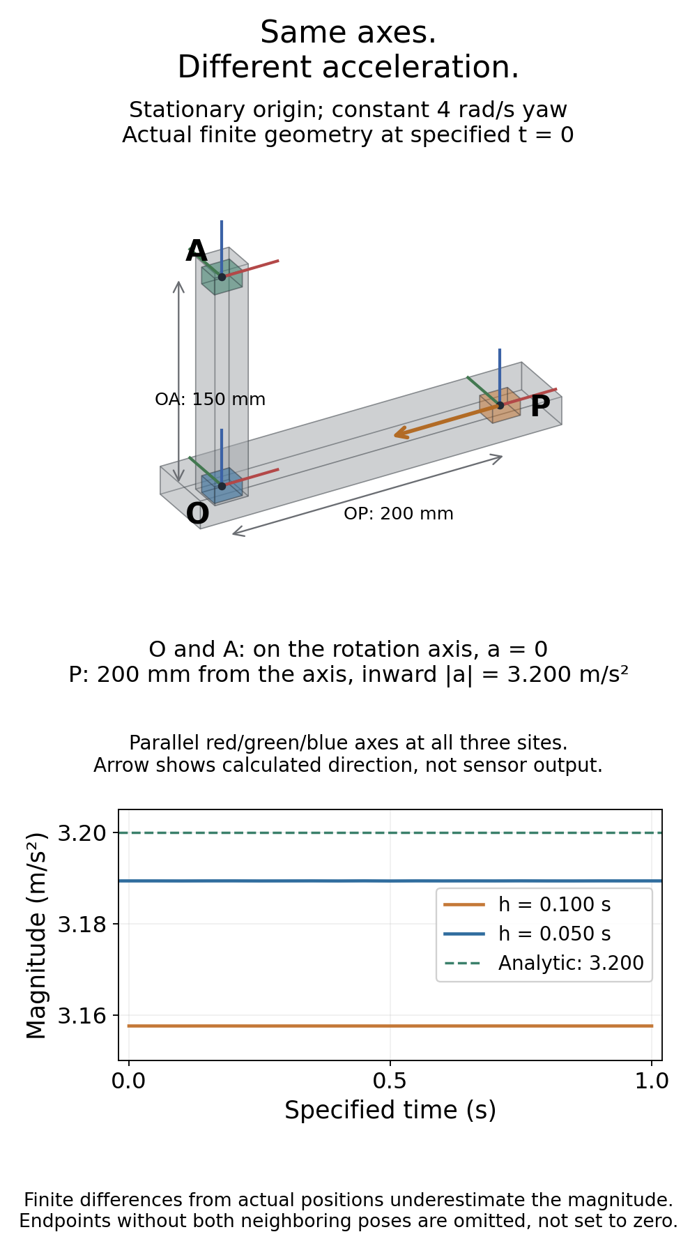
Consider a deliberately simple calculation. A rigid assembly turns about a stationary vertical axis at 4 rad/s, with no change in angular velocity. One sensor center is at the origin; another is 200 mm along body X. Their axes remain parallel to each other throughout the motion. The outer center has an inward geometric acceleration of 3.200 m/s²; the origin has zero geometric acceleration. A third center, 150 mm above the origin on the rotation axis, also has zero. Distance from the origin alone is not enough: the perpendicular distance to the rotation axis matters.
These are controlled virtual kinematic results, checked against actual finite-mesh Blender readbacks on October 6, 2026. No accelerometer, physics solver or robot produced these vectors.
The same axes can describe different points
The outer point changes velocity direction even though the angular speed stays constant. MIT’s rigid-body dynamics notes, equation 5 give the acceleration of a body-fixed point relative to another point. With a stationary origin and constant angular velocity, the expression reduces to:
a_world = omega_world × (omega_world × r_world)
Here r_world runs from the stationary origin to the sensor center. In this vertical-axis example, the result points inward with magnitude omega² × radius. The rotation matrix R maps body coordinates into world coordinates; Rᵀ a_world expresses that same point’s acceleration in body axes. It does not move the acceleration’s reference point to the origin.
At 0.400 s, the specified yaw is 1.600 rad. The outer point’s world acceleration is approximately (0.093, −3.199, 0) m/s². In body axes it is (−3.200, 0, 0) m/s². The direction changed in the coordinate description, while its magnitude and its association with the outer point stayed intact.
If the origin accelerates or angular velocity changes, the origin-acceleration and angular-acceleration terms must also be included. The constant-speed calculation below does not establish a complete lever-arm compensation method for arbitrary motion.
A stationary accelerometer does not normally report zero
Geometric acceleration is not the same quantity as raw accelerometer specific force. ROS REP-145’s official source checked on October 6, 2026, describes specific force in sensor axes, with positive Z pointing up giving approximately +g at rest. The document is marked Draft; it is a convention reference here, not evidence that a particular driver follows it.
For an ideal accelerometer convention, use f_body = Rᵀ(a_world − g_world). Choosing a uniform world gravity vector of (0, 0, −9.80665) m/s², the origin’s ideal specific force is (0, 0, 9.80665). The outer center’s is (−3.200, 0, 9.80665) in the same body axes. These are calculated vectors, not device samples. The numerical gravity value is an input, not a local gravity measurement. A gravity-removed output, a filtered estimate and a raw accelerometer channel cannot be compared interchangeably.
What the finite-mesh experiment checked
An AI-operated Blender 5.2.2 LTS experiment retained 25 specified poses in each of two cases: stationary and constant 4 rad/s yaw about world Z. The synthetic times run from −0.100 to 1.100 s in 0.050 s increments. Blender evaluated each assigned pose at static scene frame 1; these times are study inputs, not its execution clock or a measured trajectory.
Each pose includes a complete finite arm and mast, three sensor-reference boxes, and three 40 mm frame triads: eight objects, 52 evaluated vertices and 30 faces. The sensor centers and axes were recovered from actual box vertices and triad edges. All three sites share the same proper rotation. The mast, arm and reference boxes overlap by design; the geometry is not a validated mount, collision test or manufactured assembly.
An independent calculation used Rodrigues rotation to check all 2,600 world-space vertex rows, matrices, topology, normals, recovered axes and centers. It used nested cross products for analytic acceleration, and neighboring actual centers with their specified time gaps for the position differences. Source inputs, full pose logs and scene export were retained. The check accepted the expected analytic body vector near (−3.200, 0, 0) m/s² at P and zero at O and A.
This is a check of geometry and our calculations. Blender’s evaluated-mesh API did not measure acceleration or specific force. The published vectors come from the stated kinematic and gravity models. Geometry used a 1 µm comparison tolerance; axis/analytic consistency and finite-difference calculations had separately declared numerical tolerances. None is a physical IMU accuracy claim.
The two intervals produce 300 site/pose/interval records: 264 defined differences and 36 unavailable endpoint differences, kept as null rather than fabricated zeros. A stationary control gives zero geometric acceleration at all three sites. Reversing the sign of the prescribed angular velocity preserves the same inward magnitude in standalone checks. Those checks also rejected 22 deliberate corruptions and five invalid inputs, including wrong frames, units, times, gravity sign and invented sensor-output claims.
Recovering acceleration from positions leaves a time-step error
The following standard-library Python calculation samples the outer point before and after 0.400 s. Its centered second difference estimates acceleration from three positions; it does not query a sensor API.
from math import cos, sin, hypot

radius, omega, time = 0.200, 4.0, 0.400  # m, rad/s, s
def position(t):
    return (radius*cos(omega*t), radius*sin(omega*t), 0.0)

p = position(time)
exact = tuple(-omega**2*x for x in p)
for h in (0.100, 0.050):
    before, after = position(time-h), position(time+h)
    fd = tuple((before[j]-2*p[j]+after[j])/h**2 for j in range(3))
    error = hypot(*(fd[j]-exact[j] for j in range(3)))
    print(f'h={h:.3f} s: magnitude={hypot(*fd):.6f}, error={error:.6f} m/s^2')

c, s = cos(omega*time), sin(omega*time)
body = (c*exact[0]+s*exact[1], -s*exact[0]+c*exact[1], exact[2])
gravity_world = (0.0, 0.0, -9.80665)
# Yaw leaves world gravity aligned with body Z in this prescribed example.
specific_force = (body[0], body[1], body[2]-gravity_world[2])
print('analytic world:', tuple(round(x, 6) for x in exact))
print('analytic body:', tuple(round(x, 6) for x in body))
print('ideal specific force:', tuple(round(x, 6) for x in specific_force))
print('origin geometric acceleration:', (0.0, 0.0, 0.0))
With h = 0.100 s, the estimated magnitude is 3.158 m/s², about 0.042 m/s² below the analytic value. Halving h gives 3.189 m/s², about 0.011 m/s² low. For this circular trajectory, the finite-difference magnitude equals the analytic magnitude times (sin(omega*h/2)/(omega*h/2))². The discrepancy is discretization error in this noiseless calculation, not IMU bias. Smaller intervals in real noisy position data introduce other considerations that this example does not test.
When a rotating assembly’s accelerometer disagrees with acceleration at its body origin, matching the axes is only one check. Also identify the point represented by each vector, the gravity convention and the motion assumptions before attributing the difference to a sensor fault. This calculation does not evaluate a filter, calibration procedure or hardware accuracy.
For the separate problem of real sensor errors, the existing IMU bias, drift and calibration guide explains bias, scale, alignment, vibration and timing. This experiment helps keep a valid mounting-point difference out of that error budget: first name the point and axes, then the gravity convention, before interpreting a residual. Translating origins, angular acceleration, flexible mounts, nonuniform gravity, sensor filtering and estimation errors require checks beyond the two prescribed cases here.