A wheel can move throughout a sampling window without crossing the next encoder edge. If velocity is calculated from the count change in that window, the estimate is zero even though the wheel is turning. Measuring the time between edges avoids that particular staircase at steady low speed, but introduces a different limitation: a completed period describes past motion, and no new edge means no new period measurement.
The distinction matters when a low-speed velocity plot alternates between zero and large spikes. Before treating the plot as motor hunting, check the count resolution, window duration and time of the last actual edge. Texas Instruments’ eQEP application report, page 3 distinguishes counting pulses during a known interval from capturing the interval between pulses. That November 2006 report describes specific TI hardware; the calculation here illustrates the two principles without executing its peripheral, example code or timing hardware.
Fifteen rpm can appear as zero, then 37.5 rpm
Our synthetic wheel has 16 counted events per revolution and turns steadily at 15 rpm. One event represents 22.5°. These are explicitly counted events, not a manufacturer’s line count or an assumed quadrature multiplier. Using the wrong interpretation of counts per revolution would change both estimates.
The wheel starts halfway between two event positions. Observation begins at time zero with no earlier edge history. Its first four ideal crossings occur at 0.125, 0.375, 0.625 and 0.875 s. Each 100 ms count window therefore contains zero or one event:
window rpm = 60 × count change / (16 × 0.100)
One count becomes 37.5 rpm. No counts becomes 0 rpm. Yet the prescribed wheel has moved 9° during every such window. Over the whole second, four counts give 15 rpm, correctly averaging this particular interval. Lengthening a window can reduce the visible staircase, but changes the interval being averaged; it does not create sub-count position information.
An AI-operated Blender 5.2.2 LTS experiment on October 6, 2026 checked a 60 mm radius reference wheel and 16 distinct finite markers against that crossing convention. Actual evaluated vertices confirmed the prescribed marker-center alignments. The crossing times remain assigned motion inputs, not an optical encoder, interrupt trace or simulated electrical signal.
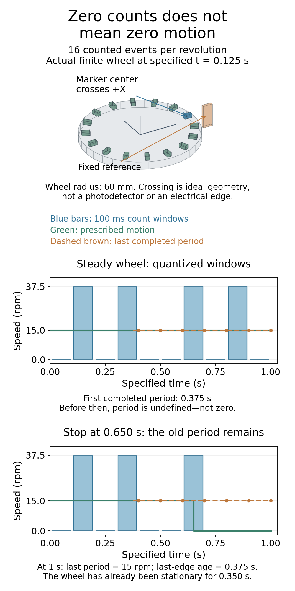
A period needs two edges—and can outlive the motion
At 0.125 s, only one edge has been observed, so this estimator has no period yet. At 0.375 s, the first completed interval is 0.250 s, giving 60 / (16 × 0.250) = 15 rpm. Its agreement with the prescribed speed depends on this ideal constant-speed example and exact timestamps. It is not a hardware accuracy result.
Now change only the motion: stop the wheel at 0.650 s. This is an abrupt prescribed stop used to examine observation limits, not a physical deceleration model. The last two edges were still at 0.375 and 0.625 s. At 1.000 s, the last available period still implies 15 rpm, although the wheel has been stationary for 0.350 s. The last edge is 0.375 s old. Retaining the numerical value does not make it a fresh velocity measurement.
The final 100 ms count window reports zero. That agrees with this prescribed stop, but the earlier steady-motion case shows why a single zero-count window cannot establish a stop by itself. A period-based estimate should remain associated with its edge timestamps; a timeout or stop-detection policy needs separate application assumptions. There is no universal timeout chosen in this example.
Finite endpoints also matter to a longer count window. The stopped wheel travels 58.5°, equivalent to 2.6 event spacings, but crosses three event positions after observation starts. A one-second count estimate is consequently 11.25 rpm, while the known one-second average motion is 9.75 rpm. Fractional positions at the interval ends explain the difference.
What the geometry and independent check establish
The native experiment assigned 24 poses to each of three cases: steady 15 rpm, the same motion until an instantaneous stop at 0.650 s, and a wheel that never moves. Common sample times included the 100 ms window boundaries, each ideal crossing and points 1 ms before and after it, and the prescribed stop. All 72 poses were evaluated at static Blender frame 1. Their timestamps describe the study schedule; they do not measure execution time or establish a physical 1 µs timer accuracy.
Each pose retained a closed 32-sided wheel, 16 finite marker boxes, a signed frame triad and a fixed reference block: 19 objects, 204 evaluated vertices and 136 faces. All rotating objects share a proper rotation about world Z. The frame and marker centers were recovered from actual vertices. An independent calculation checked all 14,688 world-space vertex rows, local geometry, matrices, face topology and normals, event geometry and the complete pose log. At each crossing, the same marker was on opposite sides of the reference direction in the before/after poses and aligned at the specified event time.
The independent event calculation used exact rational times. It checked the seven crossings across the moving cases and all 30 interval estimates, including the undefined initial period and last-edge age. Counts recovered from the actual frame phases at window boundaries agreed with the event list. The 1 µm geometric comparison tolerance is a numerical consistency limit, not an encoder resolution or hardware accuracy result.
Separate standalone checks rejected 24 deliberately corrupted records and eight invalid inputs. They also checked an event exactly on a shared window boundary and changed the initial sub-count phase: the detailed zero/one-count pattern changed even at the same steady speed. No prior native result was substituted for this experiment.
The finite geometry confirms that the prescribed wheel moves between sparse event positions. Blender’s mesh API does not measure speed, output an electrical pulse or implement the TI capture unit. The two speed estimators are our calculations under an ideal event convention.
Reproduce the two estimates from the same events
This standard-library script uses exact rational timestamps. Windows exclude their left boundary and include their right boundary, so an event on a shared boundary belongs to one window. An undefined period stays None; it is never silently converted to zero.
from fractions import Fraction as F

counts_per_rev = 16
rate = F(4)  # count crossings per second: 15 rpm
phase0 = F(-1, 2)
edges = [(F(n)-phase0)/rate for n in range(4)]

def estimates(observed_edges, query):
    seen = [t for t in observed_edges if 0 < t <= query]
    rpm = None if len(seen) < 2 else 60/(counts_per_rev*(seen[-1]-seen[-2]))
    age = None if not seen else query-seen[-1]
    return rpm, age

print('Ideal edge times (s):', [float(t) for t in edges])
for k in range(1, 11):
    start, end = F(k-1, 10), F(k, 10)
    count = sum(start < t <= end for t in edges)
    window_rpm = 60*count/(counts_per_rev*(end-start))
    period_rpm, age = estimates(edges, end)
    period_text = 'undefined' if period_rpm is None else f'{float(period_rpm):.1f}'
    print(f'end={float(end):.1f}s count={count} window={float(window_rpm):.1f} period={period_text}')

stopped_edges = [t for t in edges if t <= F(65, 100)]
last_period, age = estimates(stopped_edges, F(1))
print(f'After prescribed stop: old period={float(last_period):.1f} rpm; last-edge age={float(age):.3f}s')
print('Never moved:', estimates([], F(1)))
The count outputs switch between 0 and 37.5 rpm; the first query that can use a completed period is at 0.400 s, following the edge at 0.375 s. After the prescribed stop, the final line about that case reports the old 15 rpm value with its 0.375 s age. A wheel that never moved has no period at all.
This separates count resolution, the duration represented by an estimate, and the freshness of its supporting event. Real decoding errors, direction changes, clock quantization, timer overflow and missed edges require additional checks. None is emulated here, and the comparison does not validate a motor controller or encoder product.
For actual sensor selection, the existing robot encoder selection guide separates counted resolution, accuracy, interface and timing. Before diagnosing low-speed hunting, record the decoded counts per revolution, window boundaries, edge times and the age of the supporting data. This example covers positive one-direction motion over a finite angle range, not multi-revolution unwrapping, quadrature direction changes, missed edges, debounce, overflow or clock quantization. It does not choose gains or prove that a real motor is moving steadily.