At a cost threshold of 253, the Nav2 Collision Monitor costmap source examined here emits cell centres for costs 253 and 254. A cell with cost 255, NO_INFORMATION, follows the separate treat_unknown_as_obstacle setting. Turning that setting off omits its point; it does not clear the map or establish that the corresponding space is empty.
That difference matters when a monitoring polygon contains no observations from a blind area. Before interpreting the absence, trace the value delivered by the map, the source’s extraction settings and the points it actually supplies. A display of the robot and its monitoring region cannot answer all three questions.
This article examines Nav2 tag 1.5.2, commit 7b9be248a652224a19305469fd5e854d50512341, checked on October 6, 2026. The pinned costmap-source implementation defines the extraction behavior. The rolling configuration documentation cross-checks the parameter meanings. Rolling documentation does not establish which implementation is installed on your robot.
Why increasing the threshold cannot replace the unknown setting
The known-cost branch excludes 255 before the unknown branch is considered. Raising cost_threshold to 255 therefore removes every known-cost point, while the separate unknown flag can still emit unknown-cell centres. The examined defaults are threshold 253 and unknown handling enabled; the threshold is clamped to the range 0–255. These are source properties, not measured robot behavior.
The pinned cost constants distinguish free cost 0, maximum non-obstacle cost 252, inscribed cost 253, lethal cost 254 and no-information cost 255. For threshold 253, the source condition gives this table:
| Supplied cost | Unknown handling off | Unknown handling on |
|---|---|---|
| 0 | Omit | Omit |
| 252 | Omit | Omit |
| 253 | Emit centre | Emit centre |
| 254 | Emit centre | Emit centre |
| 255 | Omit | Emit centre |
The table describes extraction from an existing map. It is not a marking rule, clearing rule or statement about which cells a real sensor would produce. In particular, enabling unknown handling does not assert that all unknown space is physically occupied. It changes which evidence reaches this consumer.
For a diagnostic reproduction with valid byte costs, this independently authored Python form makes the separate branch visible:
def emit_point(cost, threshold, include_unknown):
    if type(cost) is not int or not 0 <= cost <= 255:
        raise ValueError("cost must be an unsigned byte")
    if type(threshold) is not int or not 0 <= threshold <= 255:
        raise ValueError("use a threshold already clamped to 0..255")
    if type(include_unknown) is not bool:
        raise ValueError("unknown handling must be boolean")
    if cost == 255:
        return include_unknown
    return cost >= threshold
This is our illustrative reproduction, not code run inside Nav2. Test the valid input domain explicitly: a value of −1 in an occupancy-grid message is not interchangeable with a supplied unsigned-byte cost in this source. The examined subscription uses nav2_msgs/msg/Costmap; trace the conversion that produced that message before comparing logs from a different representation.
An emitted point has a position, not a cell-sized solid
The source computes a cell centre as origin + (index + 0.5) × resolution in each horizontal axis, starts with source z = 0 and transforms the point to the receiving frame. It does not send the cell’s four boundaries or a 3D prism with that point. The source interface belongs to this point-producing consumer.
Consider our authored map with origin (−1.2, −1.0) m and resolution 0.1 m. Cell (4, 10) has centre (−0.75, 0.05) m. A cell index locates its centre relative to the declared origin; changing the resolution or origin changes that location even when the byte cost is unchanged.
Our comparison assigns cost 255 to that centre. At threshold 253, the off configuration omits it and the on configuration includes it. The occupied shape used for the separate geometry comparison is independently specified. We did not infer its width, height or presence from the unknown value.
Point inclusion in a polygon and finite-body overlap answer different questions. In our authored comparison, supplied cost-253 and cost-254 points enter footprint regions without either finite obstacle intersecting those regions. Conversely, a finite object can intersect the robot’s shape without a corresponding point being supplied. Inspect the conversion and observation contract before treating either result as a contact measurement.
The separate velocity-polygon experiment addresses which configured region is selected from an incoming command. The present comparison starts earlier, with which existing map cells become points. Neither comparison executes an action trigger or establishes stopping distance.
Keep missing measurements separate from missing points
A blind region, an unknown byte and an omitted source point are three different descriptions. We use an independently authored visibility proxy to make the distinction concrete: a sensor origin, a 180° forward field and finite rays to grid centres. A reverse obstacle can exist behind the sensor without appearing in those forward rays. That construction explains missing coverage; it does not implement a Nav2 observation layer.
The sensor origin itself requires special treatment. A ray aimed at the same origin has zero length and no direction to normalize. The comparison records it as not measured, rather than manufacturing a clear return. Cells outside the field are also not measured. Neither class is used to assign official cost values.
In a deployed system, a map could combine prior observations, a static source and live sensor data. Its unknown values may therefore differ from the instantaneous field of one sensor. Start with the existing costmap-layer guide when the problem is ownership, marking, clearing or inflation. For this article’s narrower question, preserve the map’s supplied values and inspect what the consumer emits from them.
What the static Blender comparison measured
We executed the authored comparison in Blender 5.2.2 LTS on October 6, 2026. It contains two separately specified obstacles and twenty static footprint poses: ten forward and ten reverse. Each footprint is a finite 0.16 × 0.30 × 0.20 m prism. We read evaluated world geometry and independently recovered the finite corners, cell-centre vertices and ray outcomes. Neither Nav2 nor a real sensor ran.
The visible obstacle is centred at (0.93, 0.47, 0.25) m, with dimensions 0.18 × 0.18 × 0.50 m. The blind obstacle is centred at (−0.75, 0, 0.25) m, with dimensions 0.08 × 0.20 × 0.50 m. Footprint centres run from x = 0.20 to 1.10 m in the forward set and −0.20 to −1.10 m in the reverse set, in 0.10 m steps. Both sets use y = 0 and footprint centre z = 0.10 m.
Coverage rays occupy a separate scene so those illustrative footprint copies cannot hide the obstacles. Both scenes use the same rigid transform: a 13° rotation about +Z and translation (0.18, −0.11, 0.04) m. Coordinates below are recovered in the authored design frame. Point inclusion tests the footprint’s XY rectangle; finite overlap separately uses the complete three-dimensional boxes.
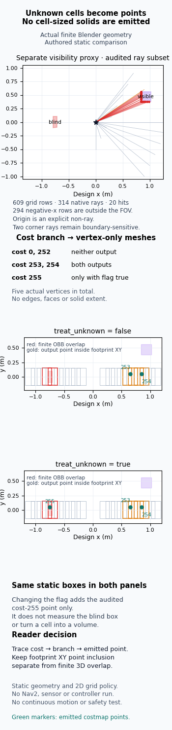
The map contains five independently assigned costs at distinct indices. We did not derive those values from ray coverage. The executed point meshes contained two vertices with unknown handling off and three with it on. Neither mesh had edges, faces or solid extent.
| Cost | Cell index | Centre x, y (m) | Point output |
|---|---|---|---|
| 0 | (14, 10) | (0.25, 0.05) | Neither configuration |
| 252 | (16, 10) | (0.45, 0.05) | Neither configuration |
| 253 | (18, 10) | (0.65, 0.05) | Both configurations |
| 254 | (20, 10) | (0.85, 0.05) | Both configurations |
| 255 | (4, 10) | (−0.75, 0.05) | Unknown handling on only |
Four forward poses, centred at x = 0.60, 0.70, 0.80 and 0.90 m, contained a known-cost point in XY but did not overlap either finite obstacle. The visible box lies laterally beyond those footprint rectangles. This demonstrates why a supplied point set should not be read as a direct reconstruction of our separately authored physical shapes.
The reverse poses centred at x = −0.70 and −0.80 m overlapped the blind box in three dimensions. With unknown handling off, both contained zero output points. With it on, each contained the same cost-255 centre in XY. Changing the flag changed the point evidence; the blind box, footprints and overlaps stayed the same. This example illustrates a possible mismatch, not a measurement of how a real costmap produces unknown cells.
The visibility grid had 609 rows. Its origin row was not a ray, and 294 negative-x rows lay outside the forward field. The remaining 314 finite native ray calls returned 20 hits and 294 misses. Independent box calculations resolved 312 of those outcomes away from corner grazing. Two rays aimed along the same nominal corner direction were boundary-sensitive: Blender returned a miss for grid (9, 6) and a hit for (12, 8). We retain that difference rather than treating either observation as proof of robust clearance. The fixed 8 micrometre numerical boundary guard is a calculation allowance, not sensor accuracy or a manufacturing tolerance.
The comparison supports the distinction between visibility, cost selection, emitted points and finite overlap. It does not measure source freshness, polygon action thresholds, controller response, braking, dynamics, continuous movement between the sampled poses, or hardware safety.
Trace the source before choosing an unknown policy
Begin with the exact deployed source type, message and version. Save a small map sample containing the cells you are trying to explain, including its byte values, indices, origin, resolution and frame. Record the threshold and unknown flag together. Comparing two configurations is useful only when the supplied map and transform are held constant.
Then inspect the emitted point coordinates in the receiving frame. A mismatch in frame, origin or resolution can put a correctly selected centre in the wrong place for the intended monitoring region. Compare the point set with the configured polygon separately from a test of physical obstacle coverage.
Do not interpret a failed source read as an empty valid observation set. In the examined implementation, missing data, stale data and a required transform failure return failure. What the caller does with that failure is another part of the application contract. A diagnostic that records only a point count loses that distinction.
The Collision Monitor configuration documentation also cautions about the latency introduced by costmap sources. A source can select the expected costs from a map that is already old. This article measures no source freshness, communication latency, controller response or hardware stopping performance.
Choose the unknown policy with the producer’s evidence, the robot’s geometry and the intended operation in view. Unknown handling on can add conservative points where physical occupancy is unconfirmed; off can omit points from places that lack observations. Neither choice repairs missing sensing or supplies a general safety guarantee. The concrete diagnostic is to trace one relevant cell all the way from its supplied byte to its centre point, then keep that result separate from what is physically present.