Nav2’s VelocityPolygon selects a configured polygon from the incoming velocity command. In the implementation examined here, it checks the sub-polygons in list order and uses the first matching region. Linear and angular limits include their endpoints. If no region matches, it logs a warning and leaves the existing polygon unchanged. It does not automatically enlarge the zone or select a polygon merely because it is named stopped or fallback.
That last detail makes coverage a configuration question with state. The same uncovered command can leave a forward-oriented zone or a reverse-oriented zone in place, depending on what matched previously. To review a configuration, you need the ordered velocity regions, the actual command entering Collision Monitor and the previous selected polygon—not just a screenshot of a zone around a stationary robot.
This article examines Nav2 tag 1.5.2, commit 7b9be248a652224a19305469fd5e854d50512341, checked on October 6, 2026. The pinned VelocityPolygon implementation is the basis for the behavior described below. The rolling configuration documentation cross-checks parameter meanings. A rolling documentation page does not establish which implementation is installed in a particular ROS environment.
Start with the command, not measured robot speed
The examined Collision Monitor caller passes the incoming command’s linear x, linear y and angular z values into its processing path. For each enabled polygon reached by that path, it calls updatePolygon(cmd_vel_in) before evaluating the configured action. This selection is based on that command input; it is not a measurement of wheel speed or an odometry-derived braking calculation.
The distinction matters while a platform accelerates, turns or responds imperfectly to a command. A configured region might select a particular polygon for x = 0.2 m/s even though the robot is not presently moving at that speed. This article does not measure that difference or any controller response. The separate short servo move experiment explains why a commanded speed limit alone does not describe a motion profile; it is a different problem from choosing a monitoring zone.
VelocityPolygon is also not a formula that computes stopping distance from speed. Each region names a polygon whose coordinates are supplied in the configuration. The polygons can be asymmetric, equal in size, or arranged for different directions. Faster commands do not inherently produce a larger polygon unless the configured regions and coordinates make that happen.
Inclusive ranges make list order observable
In non-holonomic mode, the examined code compares the command’s signed x component against linear_min and linear_max. It separately checks angular z against theta_min and theta_max. Both comparisons include the lower and upper bounds. Linear y does not participate in this mode’s region test.
The pinned example parameter file declares these velocity sub-polygons in this order:
| Example sub-polygon | Signed x interval, m/s | Angular z interval, rad/s | Polygon extent, m |
|---|---|---|---|
rotation |
0 to 0.05 | −1 to +1 | x: −0.30 to +0.30; y: −0.30 to +0.30 |
translation_forward |
0 to 1 | −1 to +1 | x: −0.20 to +0.35; y: −0.30 to +0.30 |
translation_backward |
−1 to 0 | −1 to +1 | x: −0.35 to +0.20; y: −0.30 to +0.30 |
stopped |
−1 to +1 | −1 to +1 | x: −0.25 to +0.25; y: −0.25 to +0.25 |
At x = 0.05 m/s and angular z = 0, rotation, forward and stopped all match. Rotation wins because it appears first. At x = 0 and angular z = 0, rotation, forward, backward and stopped all match, and rotation again wins. The word rotation does not add a hidden requirement for nonzero angular velocity: the numeric limits determine whether the region matches.
Moving forward ahead of rotation changes the selected polygon at the shared 0.05 boundary without changing either polygon’s coordinates. Reordering is therefore a behavior change, not cosmetic YAML cleanup. Conversely, a command just above that boundary, such as x = 0.0501 m/s, excludes the rotation interval while remaining inside the forward interval.
There is another activation detail in that example file: its top-level polygons list contains PolygonStop, while the VelocityPolygonStop block is separately declared. The presence of that block alone does not mean it is included in the list of instantiated polygons. Treat the file as an example to inspect, not a complete velocity-polygon setup already enabled by its mere existence.
A last entry is a fallback only where its limits match
The example’s stopped entry covers the same x and angular envelope already covered by the earlier entries. With the listed order and non-holonomic comparisons, it cannot win inside that envelope: an earlier region already matches. Outside x ∈ [−1, +1] m/s or angular z ∈ [−1, +1] rad/s, it also does not match. Its name and explanatory comment do not make it a universal catch-all.
The implementation’s no-match path warns and returns without assigning a new poly_. After a successful selection, that means the previously selected coordinates remain. Before any match, it leaves whatever initial polygon state exists; it does not establish a useful default zone. Our Blender illustration explicitly reset that state to empty at the beginning of each profile. That choice is not a claim that every possible Nav2 application lifecycle must start or remain that way.
For example, x = 1.2 m/s lies outside every example interval. If the preceding covered command chose the forward polygon, that uncovered command does not select the stopped polygon; it retains the forward polygon. If the preceding covered command chose the backward polygon, the same uncovered command retains the backward polygon. A description based only on the current numeric command misses that dependence on prior selection.
To make a final entry a deliberate fallback, its numeric limits and, where relevant, direction limits must cover the remaining command envelope you intend to support. Check coverage against that envelope and the preceding entries. Changing the name of the polygon supplies no coverage.
Holonomic mode changes the linear quantity and adds direction
In holonomic mode, the linear comparison uses hypot(x, y), a nonnegative speed magnitude. It also checks atan2(y, x) against the configured direction range. Angular z remains a separate inclusive constraint. At zero linear magnitude, this examined version chooses direction zero for that comparison.
For an ordinary direction interval with start ≤ end, both endpoints are included. When start > end, the code accepts directions at or beyond the start or at or below the end, allowing a region that crosses the −π/+π seam. A rear-facing interval can therefore cover directions near both +π and −π without being rewritten as one broad interval through zero.
Consider the command (x, y) = (0.06, 0.08) m/s. Its magnitude is 0.10 m/s and its direction is about 0.9273 rad, or 53.13°. In the example’s non-holonomic mode, only x = 0.06 participates in the linear region test. Our separate holonomic profile used a rear interval from +3π/4 through the seam to −3π/4, a front interval from −π/4 to +π/4, and an all-direction final region. All three used magnitude limits of 0 to 1 m/s and angular limits of −1 to +1 rad/s.
The diagonal command missed both directional regions and selected the final region in that authored profile. A reverse command (−0.1, 0) selected the wrapped rear region. At rest, the code’s chosen direction zero selected the front region. This profile is a controlled illustration, not an official default. A robot’s kinematic label does not supply suitable polygon coordinates or complete angular and velocity coverage on its own.
What changed when the observations stayed still
We ran an AI-assisted, independently authored selection model in Blender, using the source conditions above to update a real active polygon mesh. This was a Blender geometry experiment; it did not execute Nav2, ROS or TF. The scene contained four template planes, one active plane, three finite markers for observation centers and one fixed illustrative body: nine separate mesh objects.
The fixed observation centers were front (0.325, 0.15), rear (−0.325, −0.15) and side (0.10, 0.275) m in the declared base plane. The scene used a common rigid rotation and translation. For the measurements below, an independent checker reconstructed the base plane from the evaluated world vertices and matrices. It recovered each point from the center of its actual four-vertex marker, rather than substituting the requested input coordinates.
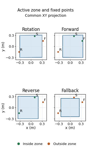
The table preserves command order within each profile. The first eleven rows use the example’s original order, the next row puts forward first, and the last four use our holonomic profile. Each profile began with an empty active mesh. For readability, forward, reverse and fallback are short polygon aliases for the example’s translation_forward, translation_backward and stopped coordinates. A retained result means no region matched and the active mesh was left unchanged.
| Profile and step | Command (x, y, angular z) | Active polygon afterward | Points inside |
|---|---|---|---|
| Original 1 | (1.2, 0, 0) | Empty, retained | No active polygon |
| Original 2 | (0, 0, 0) | Rotation | Side |
| Original 3 | (0.05, 0, 0) | Rotation | Side |
| Original 4 | (0.0501, 0, 0) | Forward | Front, side |
| Original 5 | (1.2, 0, 0) | Forward, retained | Front, side |
| Original 6 | (−0.1, 0, 0) | Reverse | Rear, side |
| Original 7 | (1.2, 0, 0) | Reverse, retained | Rear, side |
| Original 8 | (0.02, 0, 0) | Rotation | Side |
| Original 9 | (0.06, 0.08, 0) | Forward | Front, side |
| Original 10 | (0.1, 0, 1) | Forward | Front, side |
| Original 11 | (0.1, 0, 1.0001) | Forward, retained | Front, side |
| Forward-first 1 | (0.05, 0, 0) | Forward | Front, side |
| Holonomic 1 | (0.06, 0.08, 0) | Fallback | None |
| Holonomic 2 | (−0.1, 0, 0) | Reverse | Rear, side |
| Holonomic 3 | (0, 0, 0) | Forward | Front, side |
| Holonomic 4 | (0, 0, 1.0001) | Forward, retained | Front, side |
Linear components are in m/s; angular z is in rad/s. These commands were inputs to our selection model, not measured robot velocities or commands sent to a robot.
The pair of 1.2 m/s commands is the most useful comparison. After forward selection, the front point stayed inside; after reverse selection, the rear point stayed inside instead. Neither point moved. The model retained different actual mesh coordinates because of the preceding state. Reordering at 0.05 m/s produced another visible difference: the front point was outside the original rotation selection and inside the forward-first selection.
The reconstructed distance from the front point to the rotation boundary was approximately 25 mm, with that point outside. It was also approximately 25 mm from the forward boundary, this time inside. Under reverse selection it was outside by approximately 125 mm to the nearest finite edge. In the holonomic fallback state, front and rear were outside at approximately 75 mm from the boundary, while side was outside at approximately 25 mm. These rounded distances describe points relative to a zone boundary. They are not robot-to-obstacle clearance, braking margins or evidence that any pose is safe.
The separate checker cross-checked finite-edge halfspaces with ray crossing and required each classified point to lie beyond a fixed 10 micrometre boundary guard. All observation classifications reported here met that requirement. The run retained 40 complete geometry captures around 19 transitions—16 commands and three resets—producing 1,560 CSV vertex rows. Those are repeated records of the same nine mesh objects, not 1,560 unique vertices or separate trials. Templates, observation markers and the illustrative body remained unchanged; only the active mesh was reset or rewritten.
A point inside a zone is not a stop test
The examined point-counting implementation tests observation points against a polygon. Its containment helper uses a ray-crossing algorithm. This is not a test of intersection between complete finite obstacle and robot meshes. Our three small markers represent point centers; their solid extent was not substituted for those points in the classification.
Velocity-range endpoint inclusion also does not establish a general rule for a point exactly on a polygon edge. Our observations were deliberately away from edges, and the numerical guard kept those two questions separate.
A point inside a zone does not, by itself, prove that Collision Monitor would stop the robot. The configured minimum point count and action logic are separate inputs. The pinned velocity-polygon example specifies six minimum points, while our illustration had three declared observations; these counts are not an executed action-trigger test. The LiDAR angular sampling experiment covers the separate issue of whether sensor sample directions yield observations of a small object at all.
Review a velocity-polygon configuration as a selection contract
First, confirm that the velocity-polygon block is actually named in the node’s polygon list and that the input topic is the command you intend to monitor. Then read the sub-polygon list in order, using signed x in non-holonomic mode or magnitude and direction in holonomic mode. Include exact linear, angular and direction boundaries in that review.
Trace uncovered commands with more than one preceding selected zone. If the intended final entry is a fallback, test its coverage rather than relying on its name. Finally, check which observation points lie inside the selected geometry and which configured thresholds and action rules use those points.
The Blender experiment made order, retained state and point classification visible in actual changing meshes. It did not measure sensor freshness, processing latency, stopping distance or hardware response, and it provides no safety certification. For this selection question, the practical result is specific: inspect the previous selected polygon whenever the current command lies outside every configured region.