Motion planning searches for a valid way to connect a start and goal through a constrained space. Trajectory optimization adjusts a finite representation of states and controls to reduce costs while satisfying constraints. Sampling-based planning is often better at discovering different routes; local trajectory optimization is often better at refining a useful initial route.
The terms overlap in software and research, but the distinction helps system design. A geometric path may omit time and dynamics. A trajectory includes time, and a dynamically feasible trajectory respects equations of motion, control and state limits. Neither result guarantees accurate execution without feedback and an updated environment model.
Use this guide with the robot simulator comparison and kinematics and dynamics guide. Evaluate the complete pipeline from world model to tracked hardware motion.
Define path, trajectory and policy separately
A path is a sequence or continuous curve through configuration or state space without an execution schedule. Time parameterization creates velocity and acceleration references. A trajectory can include state and control over time. A policy maps observed state to action and can react across a region rather than only replay one nominal motion.
These outputs support different claims. Collision-free waypoints are not necessarily dynamically feasible, and an open-loop optimized trajectory is not automatically robust. State the planned space, time representation, control variables and feedback used in execution.
Sampling-based planning searches connectivity
OMPL implements randomized geometric and control-based planners. Its planner documentation shows distinct families and problem assumptions. Methods such as RRT and PRM sample states and connect valid regions rather than optimizing every trajectory variable from one initial guess.
Sampling can explore narrow alternatives and different homotopy classes, but success and quality depend on state space, validity checks, range, goal bias and time budget. A returned path may be jagged or sparse. Post-processing and time parameterization are normally needed before execution.
| Property | Sampling-based planning | Trajectory optimization | Hybrid use |
|---|---|---|---|
| Main strength | Explore connectivity | Refine costs and constraints | Search then smooth |
| Initialization | Start and goal plus sampler | Initial trajectory or guess | Planner supplies seed |
| Global alternatives | Often better coverage | Usually local | Try several seeds |
| Dynamics | Geometric or control variant | Can enforce directly | Select by task |
| Output quality | May need smoothing | Cost-dependent smoothness | Verify final trajectory |
Collision checking quality controls planner validity
MoveIt’s motion-planning documentation explains its use of planning plugins and collision models. A planner is only as correct as robot geometry, attached objects, environment updates and the interpolation used between checked states.
Coarse edge checking can miss a thin obstacle even when sampled endpoints are valid. Include swept volume, tool geometry and self-collision. Record collision resolution and scene timestamp. Add margins for calibration error, perception uncertainty, tracking error and stopping distance rather than treating a zero-distance mathematical boundary as operational clearance.
Trajectory optimization turns motion into a nonlinear program
The MIT trajectory-optimization chapter formulates finite-horizon state and input trajectories with dynamics, objectives and constraints. Direct transcription or collocation creates finite decision variables at knot points and enforces discretized dynamics between them.
Costs can penalize duration, effort, jerk, tracking error or risk. Constraints can enforce start and goal, collision distance, state and input bounds, contact and dynamics. The result depends on transcription, solver tolerance and discretization. Constraint satisfaction at knots does not automatically prove continuous-time validity between knots.
Initialization determines which local solution is found
Many trajectory problems are nonconvex because of obstacles, rotations, contact and nonlinear dynamics. A local solver can converge to the route encoded by its initial guess, stop at a poor local minimum or report infeasible even though another route exists.
Use a sampling planner, human demonstration, previous solution or coarse optimization as a seed. Run several topologically different seeds for hard scenes. Track termination status, objective, constraint residual and time. A numerically smaller cost is irrelevant if the trajectory violates a physical assumption.
Geometric planning and kinodynamic planning differ
Geometric planning searches configurations and usually assumes that a later stage can time the path. It is effective for many manipulator tasks when dynamics are not the main bottleneck. Kinodynamic planning searches state and control under differential constraints, which matters for vehicles, underactuated systems and high-speed motion.
Choose the state space from the plant, not from software convenience. A car cannot translate sideways even if a geometric point path permits it. A heavy arm can follow a geometric route slowly but not at an arbitrary acceleration. Validate feasibility after the final timing stage.
| Validation layer | Question | Metric | Failure evidence |
|---|---|---|---|
| Geometry | Is the swept robot collision-free? | Minimum distance | Continuous collision test |
| Kinematics | Are joints and singularities acceptable? | Limit and condition margin | Full-path sample |
| Dynamics | Can the plant create the motion? | Torque and control residual | Model replay |
| Timing | Are rate and acceleration bounded? | Peak and continuity | Interpolated profile |
| Execution | Can feedback track safely? | Error and stopping distance | Hardware trials |
Hybrid pipelines use each method for its strength
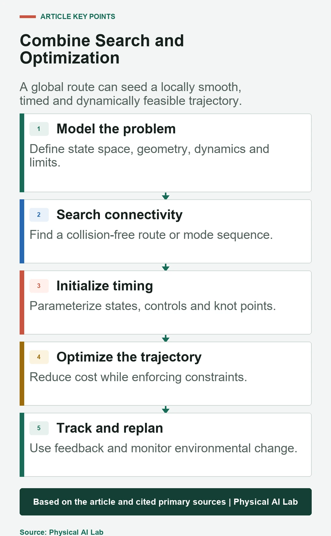
A common pipeline finds a collision-free route with a sampling planner, smooths or shortcuts it, assigns time, and optimizes a trajectory with dynamics and task costs. Another approach repeatedly replans locally while retaining a global guide. The stages must share frames, geometry and constraints.
Recheck collision and limits after every smoothing or optimization stage. A shortcut can cut into an obstacle, while timing can expose velocity or torque problems. Preserve the original and final path, solver configuration and scene version for diagnosis.
Simulation tests the algorithm but not every hardware effect
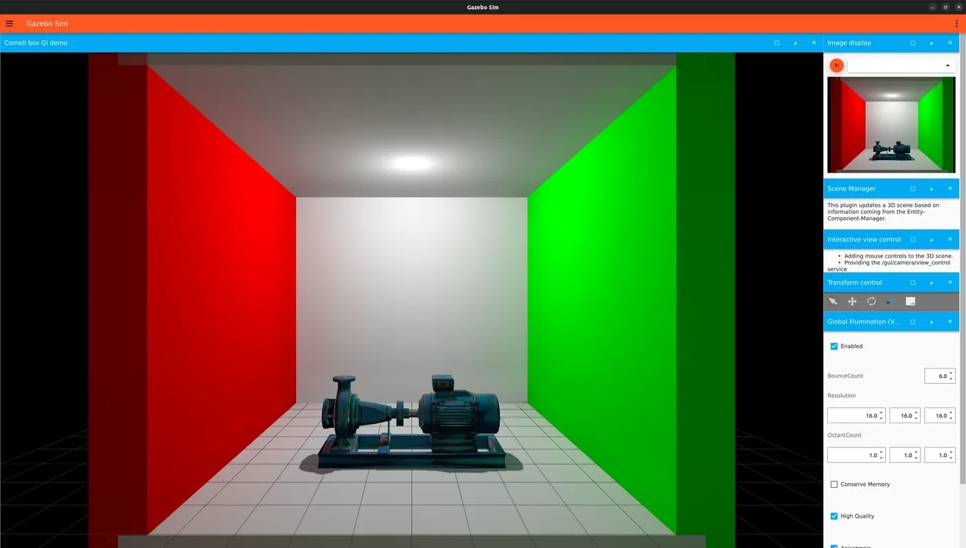
Gazebo Sim is an open robotics simulator for modeled sensors, dynamics and environments. The project repository supports repeatable integration tests, scene changes and collision experiments. Simulation is valuable for broad failure exploration before commanding hardware.
Contact, friction, actuator saturation, latency, calibration and deformable obstacles may differ from reality. Validate the planner’s geometry against the real tool and fixtures, then begin hardware tests at reduced speed and energy. Use observed tracking error and stop distance to set margins.
Dynamic environments require age-aware replanning
A collision-free trajectory can become invalid after an obstacle moves or perception changes. Record the age of the world state used to plan. Monitor execution against the current scene and trigger slowing, stopping or replanning before remaining clearance is consumed.
Replanning latency includes sensing, fusion, scene update, planner time, trajectory validation, controller handoff and actuator response. Measure the complete chain and its jitter. A fast median solve does not justify high speed if tail latency is unbounded.
Benchmark both solve quality and execution outcome
Use varied starts, goals, obstacle layouts, seeds and time budgets. Measure success, solve time distribution, path length, clearance, smoothness, constraint residual, torque margin and replans. Separate planning failure, validation failure and controller execution failure.
On hardware, add tracking error, stop distance, contact, cycle time and recovery. Retain unsuccessful trials rather than reporting only the best path. The best planner is the one that meets the task and evidence envelope consistently, not the one with one fastest demonstration.
- Define the planned state, time and control variables.
- Validate edges continuously at an explicit resolution.
- Use multiple seeds for nonconvex optimization.
- Recheck constraints after every post-processing stage.
- Measure world-state age and end-to-end replanning latency.
Frequently asked questions
Is motion planning the same as trajectory optimization?
No. Motion planning broadly seeks a valid connection, while trajectory optimization numerically refines a parameterized timed motion under costs and constraints. They can be combined.
Does a collision-free path include timing?
Not necessarily. A geometric path may have no velocity or acceleration. Time parameterization and dynamic validation are separate steps.
Why does trajectory optimization need a seed?
Nonconvex objectives and constraints create local solutions. The initial guess often determines the route and whether the solver converges.
Can OMPL enforce dynamics?
OMPL has geometric and control-based planners. The selected planner and state-propagation model determine whether differential constraints are represented.
What must be checked before hardware execution?
Check scene age, continuous collision, joints, singularities, speed, acceleration, torque, interpolation, controller interface, stopping behavior and operational margins.
Motion Generation Boundary Note
A solver success flag is not proof of continuous collision freedom, physical feasibility or safe execution. Validate the final interpolated trajectory with current geometry, dynamics, feedback and measured stopping behavior.