A two-U-joint shaft can return to the correct output angle after one complete input revolution and still move unevenly throughout that revolution. In the ideal coplanar example below, equal 25° bends with aligned middle-shaft yokes give 1° of output motion for every 1° input step. Turning one middle yoke by 90° changes that output step to between 0.8214° and 1.2174°. Keeping the yokes aligned but changing the second bend to 15° leaves a smaller variation. Both assembly checks matter.
This is a geometric comparison for someone arranging two single Hooke-type universal joints between fixed shaft axes. On October 5, 2026, we ran this AI-operated virtual comparison in Blender 5.2.2 LTS and independently audited all 1,083 evaluated configurations. The ranges below come from the modeled shaft and bearing axes, not measured motor speeds. No physical joint was operated. The selected 25° bend is an illustrative input, not an operating-angle recommendation.
First identify the two different angles
The bend angle is the angle between the shaft axes connected by one joint. Phasing is the relative clocking of the two yokes attached to the intermediate shaft. Changing shaft placement changes the bends; turning a yoke about the intermediate shaft changes phasing. Correcting one does not necessarily correct the other.
Belden’s U-joint phasing guidance calls for coordinated yoke orientation and suitable coplanar shaft alignment, with equal operating angles for the two-joint relationship described there. It also distinguishes the motion at the outer shafts from the varying motion of the intermediate shaft. These are manufacturer installation principles; the calculation here isolates their geometric consequences rather than validating a product or its load rating.
Our phase zero means that the two bearing-axis lines on the intermediate shaft are parallel. A directed marker would reverse at 180°, but the physical bearing line would be unchanged. Belden also describes inward-facing yokes using a 180° convention. Those references should not be compared as bare numbers without identifying which yoke face or bearing line each uses.
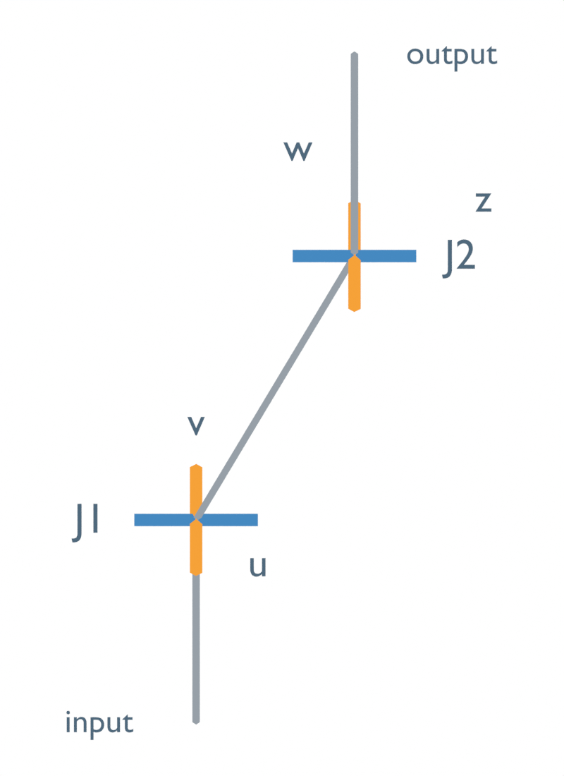
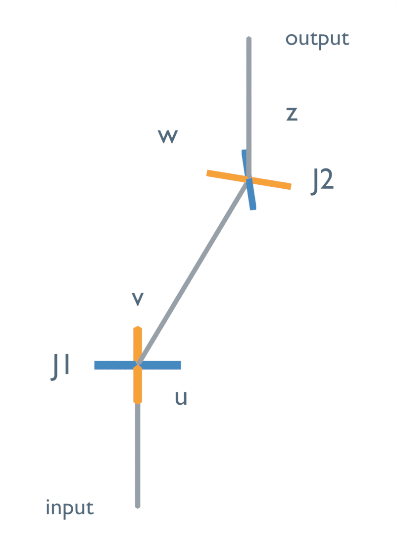
Gray bars represent the fixed shaft axes. Orange v and w belong to the intermediate shaft; blue u and z belong to the outer shafts. Each joint keeps its two bearing directions perpendicular. The bars show those directions, not fork clearances or a contact simulation.
Compare a whole revolution, not just the finishing marks
The first joint bends by 25° in all three cases. The intermediate shaft is 300 mm between joint centers. Each arrangement lies in one plane. With equal bends, the input and output axes are parallel; reducing the second bend to 15° changes the output axis as well. This is a fixed layout comparison, not a claim that the endpoint shaft orientation remained unchanged.
The input is sampled from 0° through 360° in 1° steps. There are 361 poses and 360 intervals. Output angles are unwrapped across complete revolutions, then the initial output angle is subtracted. That removes the different initial index of the misphased case without hiding its variation during the cycle.
| First / second bend | Middle bearing-line phase | Smallest output step per 1° input | Largest output step per 1° input | Total output rotation |
|---|---|---|---|---|
| 25° / 25° | 0°, aligned | 1.0000° | 1.0000° | 360° |
| 25° / 25° | 90° | 0.8214° | 1.2174° | 360° |
| 25° / 15° | 0°, aligned | 0.9383° | 1.0658° | 360° |
These are native-readback finite-angle increments, independently checked against the ideal equations and rounded to four decimals. They are interval averages of the angle relationship, not exact instantaneous speed extrema. If an ideal input shaft were driven at constant angular speed, this relationship would determine the corresponding ideal output-speed variation. No physical constant-speed drive was run here.
Positive values place the output ahead of its matching input displacement; negative values place it behind. The 90° phase case’s initial output orientation is removed from this comparison, so its curve shows the variation during the turn. Returning to zero at the end does not remove the deviations between the endpoints. The near-zero aligned curve contains only tiny numerical readback variation.
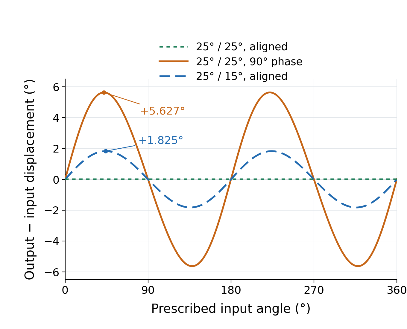
All three cases finish at the same relative output angle. A mark checked only after a full turn would miss the difference. In the 90° case, the measured model output displacement departs from the input displacement by as much as about 5.63° at the sampled poses; the unequal-bend case reaches about 1.82°.
The middle shaft is not uniform even in the equal, correctly phased case. Its native-readback step spans about 0.9063°–1.1034° for each 1° input step in all three arrangements. The second joint can cancel the variation at the output while the intermediate member still experiences varying angular motion. Output cancellation therefore cannot establish the behavior of every component in the assembly.
Reproduce the ideal relationship
Let θ be the input angle, ψ the intermediate angle, χ the output angle, β₁ and β₂ the two bends, and δ the middle bearing-line phase defined above. The cross-bearing axes at each joint must remain perpendicular. In our coplanar coordinate convention that gives:
ψ = atan2(sin θ, cos β₁ · cos θ)
χ = atan2(cos β₂ · sin(ψ + δ), cos(ψ + δ))
Using atan2 preserves the quadrant. Unwrapping then preserves the full turn. A single-argument arctangent of a quotient can lose which half of the rotation a pose belongs to.
The following Python uses only the standard library. Its output reproduces the table; each reported increment is output degrees per one input degree.
from math import atan2, cos, sin, radians, degrees, pi

def unwrap(values):
    out = [values[0]]
    for value in values[1:]:
        out.append(out[-1] + (value - out[-1] + pi) % (2*pi) - pi)
    return out

for b1_deg, b2_deg, phase_deg in [(25, 25, 0), (25, 25, 90), (25, 15, 0)]:
    b1, b2, phase = map(radians, [b1_deg, b2_deg, phase_deg])
    theta = [radians(i) for i in range(361)]
    psi = unwrap([atan2(sin(t), cos(b1)*cos(t)) for t in theta])
    chi = unwrap([atan2(cos(b2)*sin(p+phase), cos(p+phase)) for p in psi])
    increments = [degrees(b-a) for a, b in zip(chi, chi[1:])]
    middle = [degrees(b-a) for a, b in zip(psi, psi[1:])]
    print(f'{b1_deg}/{b2_deg}, phase {phase_deg}: '
          f'output {min(increments):.4f}..{max(increments):.4f} deg per 1 deg input; '
          f'net {degrees(chi[-1]-chi[0]):.1f} deg; '
          f'middle {min(middle):.4f}..{max(middle):.4f}')
At equal bends and zero phase, substituting the first relation into the second cancels the angle distortion. Clocking the intermediate yokes changes the second relation’s input phase. Unequal bends leave different cosine factors, so alignment alone cannot cancel the distortion.
The native construction solved bearing directions using cross products, then measured evaluated world coordinates at every prescribed input angle. An independent script used the equations above to reconstruct all marker positions and checked all seven evaluated box meshes per configuration, including their vertices, transforms and end faces. The greatest position discrepancy was below 0.000050 mm and the greatest angular discrepancy below 0.000059°. Tiny readback variation around the equal-case ideal 1° increment is numerical; it is not a manufactured-joint tolerance. Frames index angles, not time or RPM.
The equality controls also matter. With zero bends, arbitrary phase changes the initial index but the output displacement still advances uniformly. A 180° reversal of our directed middle marker preserves the aligned bearing-line result. Exactly 90° shaft bends are excluded because this construction becomes singular at some input poses. The model is not an instruction to operate hardware near that boundary.
What to check in an assembly drawing
Start by identifying the actual shaft axes and measuring both true bend angles. Then mark the two intermediate-shaft bearing-axis lines and compare their clocking around that shaft. Inspect the same physical features at both ends; visual symmetry of the outside yoke shape is an unreliable substitute for a defined reference.
Next compare motion across a full input revolution. A final 1:1 revolution count is insufficient, and aligning the middle yokes is insufficient if the selected layout leaves unequal bends. If an output mechanism needs precise indexing, distinguish an initial angular offset from periodic angular error before choosing a correction.
These checks address a different question from gear center-distance and contact: whether the chosen joint arrangement preserves angular progression between shafts. If the output later drives a linear mechanism, its own crank or yoke endpoint timing is another transformation to evaluate.
The model uses fixed, coplanar shaft axes and ideal rigid bearing directions. It omits yoke interference, joint clearances, bearing friction, inertia, support compliance, torque and wear. It is not a centered double-Cardan hardware design or a guarantee that a real two-joint transmission is suitable at a particular speed. Use the geometric result to correct the layout or clocking question, then apply the actual joint manufacturer’s conditions to the proposed hardware.