Robot sensor fusion combines measurements with different rates, frames, noise and failure modes into an estimate of position, velocity, orientation, bias or another state. The goal is not to average every input. It is to use a process model and uncertainty so complementary evidence corrects drift without allowing bad or duplicated measurements to dominate.
Time alignment, coordinate transforms and covariance are often more important than the choice between an extended and unscented Kalman filter. A precise sensor with a stale timestamp or wrong extrinsic can degrade the estimate. More sensors help only when their relationships and correlations are modeled honestly.
Read this with the robot sensor guide and calibration workflow. Treat estimator output as a model-dependent estimate with uncertainty, not as independent ground truth.
Fusion combines prediction and measurement correction
A state estimator propagates the previous state through a motion or process model and increases uncertainty according to process noise. When a measurement arrives, it predicts what that sensor should observe, compares the innovation and applies a correction weighted by uncertainty.
This structure supports sensors that arrive asynchronously. A fast IMU can propagate orientation and velocity, while slower wheel, lidar, camera or satellite observations constrain drift. The output rate can be high even when absolute measurements are intermittent, but uncertainty must grow during unobserved motion.

Timestamp means measurement time, not arrival time
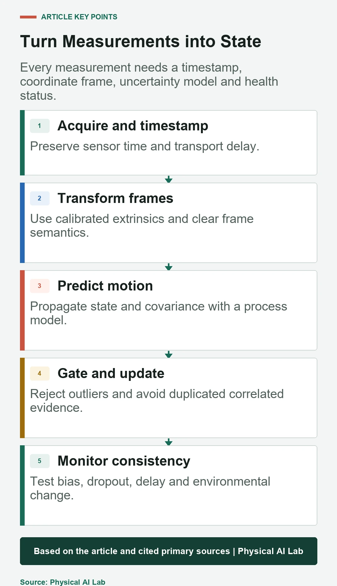
A sensor message can be captured, processed, queued, transported and received at different times. Using host arrival time as capture time turns motion during latency into spatial error. Preserve hardware time where possible and measure the mapping between device clocks and the estimator clock.
Characterize fixed offset, jitter and drift. Correct known delay or process out-of-sequence measurements with an estimator designed for them. Log capture, publication and reception time separately. An accurate calibration measured at rest can still fail on a moving robot if streams are misaligned.
| Data field | Meaning | Failure if wrong | Verification |
|---|---|---|---|
| Capture time | Physical measurement instant | Motion-dependent bias | Triggered motion test |
| Frame ID | Coordinate basis | Rotated or shifted estimate | Known-direction input |
| Covariance | Expected uncertainty | Over- or underweighting | Innovation statistics |
| Sequence or source | Measurement identity | Duplicate evidence | Message tracing |
| Health state | Validity and mode | Silent bad updates | Fault injection |
Coordinate frames require calibrated transforms
ROS REP-105 defines common mobile-robot frame roles such as map, odom and base_link. The map frame can jump after global correction, while odom is expected to remain locally continuous. Mixing their semantics creates controller discontinuity.
Each sensor extrinsic must map its measured quantity into the estimator convention with the correct rotation, translation and handedness. IMU orientation, angular velocity and acceleration need a documented frame and gravity convention. Recalibrate after sensor movement, collision or structural service.
Covariance tells the estimator how much to trust
Measurement covariance represents uncertainty, including cross-axis relationships when modeled. Process noise represents mismatch between assumed motion and the real system. Values that are artificially small make a sensor dominate; values that are too large prevent useful correction.
Estimate noise and bias under stationary, moving and environmental conditions. Then inspect innovations rather than tuning only for a visually smooth path. A smooth but biased estimate can be worse for control than a slightly noisy honest estimate. Update parameters when tires, payload, lighting or surface change.
| Symptom | Likely cause | Evidence | Adjustment |
|---|---|---|---|
| Estimate follows one sensor exactly | Covariance too small | Innovation and gain | Re-estimate noise |
| Correction barely changes state | Covariance too large | Residual persists | Check units and covariance |
| Slow drift | Bias or unobserved state | Long reference run | Model bias or add observation |
| Oscillation after updates | Delay or frame error | Velocity-correlated residual | Fix time and transform |
| False confidence | Correlated duplicate input | Covariance shrinks too fast | Remove or model correlation |
EKF and UKF make different nonlinear approximations
The ROS robot_localization documentation provides EKF and UKF state-estimation nodes for multiple sensor sources. An EKF linearizes models with Jacobians, while a UKF propagates selected sigma points through nonlinear functions.
A UKF is not universally more accurate, and an EKF is not universally sufficient. Model quality, noise, timing, observability and implementation dominate many deployments. Compare them on the same recorded data with the same state, frames and covariance, then evaluate consistency, latency and computation.
Correlated measurements must not be counted twice
Wheel odometry may already combine left and right encoders; visual odometry may reuse an IMU; a global pose may be computed from the same local estimate being fused. Treating derived outputs and their source measurements as independent makes covariance shrink without new information.
Trace measurement lineage. Fuse the most appropriate raw or derived level once, or model cross-correlation with a suitable estimator. Avoid feeding the estimator’s own output back as a fresh measurement. Document which state components each source contributes.
Innovation gating contains outliers
The innovation is the difference between an incoming measurement and its predicted value. Normalize it by expected innovation covariance and reject or downweight values outside a validated threshold. This can contain multipath, feature mismatch, wheel slip or momentary sensor faults.
A gate cannot fix persistent bias or a wrong frame. Monitor rejection rate by sensor and environment. Excess rejection may signal a broken model; no rejection may mean thresholds are ineffective. Define recovery after a long outage or a large global relocalization.
Bias and observability determine long-term drift
An IMU bias integrates into velocity and position error. Wheel radius or scale error accumulates distance bias. Whether these quantities can be estimated depends on motion and external observations. A state can be mathematically included yet remain unobservable during the available trajectory.
Design calibration motions that excite relevant axes and compare against an independent reference. Monitor covariance and parameter correlation. Do not lock a poorly observed bias to a confident value simply to make the estimate look stable.
Fusion and SLAM have overlapping but different scopes
SLAM estimates a map and robot trajectory using environmental observations, while a general state estimator can fuse odometry, IMU, global pose and other measurements without building a map. OpenCV calibration tools address camera geometry that both systems may rely on.
A SLAM pose can be one measurement source for a local filter, but loop-closure jumps must be handled with correct frame semantics. Controllers often prefer a locally continuous odom estimate while global planning uses map alignment. Define the boundary to avoid feedback loops and duplicated evidence.
Validate with reference data and injected failures
Use stationary, straight, turning, stop-start, uneven-surface and repeated-loop tests. Compare position, orientation, velocity, bias, covariance and innovation with an independent reference where possible. Evaluate start-up, warm-up and long-duration drift rather than one short route.
Inject sensor delay, dropout, bias, outliers, duplicated messages, transform error and wheel slip. Verify uncertainty growth, rejection, recovery and controller behavior. Store raw data and configuration so failures can be replayed. A filter is ready when it remains bounded and honest under expected faults, not merely when its path looks smooth.
- Preserve capture time and measure transport delay.
- Calibrate every sensor frame and gravity convention.
- Tune uncertainty from data and inspect innovations.
- Trace correlations and avoid double counting.
- Test dropout, bias, outliers and recovery with control connected.
Frequently asked questions
Will adding more sensors always improve accuracy?
No. Extra sensors help only when their time, frame, covariance, bias and correlation are modeled and their measurements add independent information.
Is a UKF always better than an EKF?
No. The better choice depends on model nonlinearity, computation and implementation; timing, calibration and uncertainty errors often matter more.
How should covariance be selected?
Begin with measured noise and bias across relevant conditions, include process-model mismatch, then check innovation consistency and independent reference error.
How serious is camera-to-IMU timing error?
It can create pose and velocity bias proportional to motion, especially during fast rotation or vibration. Measure end-to-end timestamp offset and jitter.
Should the filter stop when one sensor disappears?
Not always. It can predict with remaining inputs, but uncertainty must grow and the system needs a bounded slow, stop or degraded policy when observability is lost.
State Estimation Boundary Note
Estimator output and covariance depend on model and sensor assumptions and are not independent ground truth. Validate time, frames, correlations, bias, delay and faults with an external reference and the connected controller.