A drum calibration based only on the bare shaft radius can be wrong as soon as the cable winds at a different radius. In my Blender comparison, one turn of the captured finite cable centerline measured about 75.648 mm at a 12 mm winding radius and about 150.876 mm at a 24 mm winding radius. The larger-radius static specimen contained almost twice the finite section-centroid polyline length for the same recovered turn count.
The ratio was about 1.99445 rather than exactly 2. The centerline radius doubled, but the authored helix kept a fixed 6.5 mm axial pitch per turn. The measured curve was also a 64-chord polygonal centerline, not an exact smooth helix. Those details are small enough to disappear in a sketch and large enough to matter when deciding what a “millimetres per turn” constant actually represents.
I created and measured six independent static models in an AI-operated Blender 5.2.2 LTS session on October 8, 2026. They compare half, one, and one-and-a-half turns at 12 and 24 mm prescribed centerline radii. This was a geometric experiment. It did not rotate a drum, wind a physical cable, read an encoder, or measure payout under tension.
Radius belongs to the cable centerline, not just the shaft
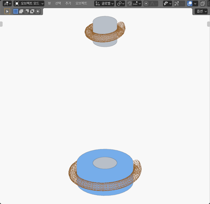
The gray drum core has a 9 mm radius. The orange-brown tube has a 3 mm section radius. In the first state, its prescribed centerline radius is 12 mm; in the second it is 24 mm. The blue annular solid shown in the larger-radius cells is an authored envelope with a 21 mm outer radius. It illustrates a larger winding state, but it is not a simulated history of layers building up.
Those numbers define three different radii that should not be mixed:
- 9 mm is the core radius.
- 12 or 24 mm is the cable centerline radius used for the length calculation.
- 15 or 27 mm is the prescribed outermost radial surface envelope of the 3 mm tube at those centerline states.
For length per turn, the centerline radius is the relevant geometric input. Using the 9 mm shaft radius would describe neither captured cable state. Using 15 or 27 mm would instead follow the tube’s outer surface, which is also not the measured centerline.
The same distinction appears in practical routing problems. The moving-pulley cable experiment maps cable take-up to carriage travel along a chosen route. This drum experiment asks a narrower question: how much finite centerline length corresponds to a recovered turn at a prescribed winding radius. Combining those two mappings would require a complete mechanism model; neither article demonstrates a physical cable drive.
Six static curves recovered the same turn counts
Each strand was authored as a closed 12-sided tube around a helical centerline. The model used 64 intervals per turn and a 6.5 mm axial pitch per turn. The six cases covered 0.5, 1.0, and 1.5 turns at each radius.
I did not take the object origin or the input turn label as the result. The drum axis was recovered from the two actual 32-vertex core-cap centroids. For every cable section, the 12 actual section vertices were averaged to recover its center. Those centers were projected around the recovered axis, and each positive angular increment was calculated and unwrapped before summing the turn count.
The same actual section centers supplied the length. I summed the three-dimensional chord between every neighboring pair. That makes the reported quantity the finite polygonal centerline length represented by the captured mesh. It is not the tube’s material neutral axis, the length of a physical cable under tension, or an encoder-derived payout.
All six cases recovered their authored turn counts: 0.5, 1.0, and 1.5 within the experiment’s arithmetic bounds. Their actual recovered pitch was approximately 6.5 mm per turn. The half-turn and one-and-a-half-turn cases finish at the same wrapped angular position relative to their starts. The latter contains one additional revolution. An endpoint angle alone would alias those two cases; summing every ordered angular increment distinguishes them.
Measured length scaled with radius across all three turns
| Authored turns | Centerline radius | Finite centroid-chord length bounds | Recovered turns | Length per recovered turn bounds |
|---|---|---|---|---|
| 0.5 | 12 mm | 37.823–37.825 mm | 0.500 | 75.647–75.649 mm/turn |
| 0.5 | 24 mm | 75.437–75.439 mm | 0.500 | 150.875–150.877 mm/turn |
| 1.0 | 12 mm | 75.647–75.649 mm | 1.000 | 75.647–75.649 mm/turn |
| 1.0 | 24 mm | 150.875–150.877 mm | 1.000 | 150.875–150.877 mm/turn |
| 1.5 | 12 mm | 113.470–113.473 mm | 1.500 | 75.647–75.649 mm/turn |
| 1.5 | 24 mm | 226.313–226.315 mm | 1.500 | 150.875–150.877 mm/turn |
The reported model bounds include the segment arithmetic allowances. I rounded every lower endpoint downward and every upper endpoint upward to 0.001 mm; the recovered turn counts are rounded for display. These intervals do not enclose uncertainty in a physical cable. The table shows two useful consistency checks. First, dividing each captured length by its independently recovered turn count gives nearly the same per-turn interval for all three samples at a given radius. Second, changing from 12 to 24 mm almost doubles the result at every turn count.
The finite result is slightly shorter than the corresponding smooth-helix calculation. For one ideal smooth turn, sqrt((2πR)^2 + pitch^2) gives approximately 75.677884 mm at 12 mm and 150.936472 mm at 24 mm. The actual model joins 64 straight center-to-center chords per turn, so each polygonal curve cuts slightly inside the smooth arc. Those nominal formula values are a mathematical cross-check only; I did not substitute them for the captured mesh measurements.
The per-segment arithmetic allowance was 10 nanometres for length and 1e-12 radians for each angular increment. These are bounds for reproducing calculations from this authored geometry, not physical measurement accuracy or manufacturing tolerances. The larger coordinate-correspondence allowances used to validate mesh construction are a separate check and should not be added to the per-turn numbers as if they described a real cable.
A smooth formula is a check, not the captured answer
The near-doubling result is easy to anticipate from circumference, but a useful calibration still needs its assumptions stated. If pitch were zero and the measured path were a perfect circle, doubling radius would double length per turn exactly. Here pitch remains fixed while the circumference term doubles. The pitch contribution therefore becomes a smaller fraction of total length at the larger radius, producing the observed ratio of about 1.99445.
Sampling also matters. As a mathematical approximation, straight chords approach the smooth helix with finer sampling. I kept 64 intervals per turn in this run and did not perform a resolution-convergence experiment. A calibration derived from one discretization should identify whether it is using chord length, an analytical curve, or a physical measurement. Mixing them can make a small numerical difference look like a mechanical anomaly.
Blender’s Circle primitive documentation was checked on October 8, 2026 and supports the limited modeling vocabulary used here: radius, vertex count, a finite polygon, and a fill choice. I authored the drum loops and cable sections directly rather than claiming that a Circle operator produced or validated the winding model. The manual does not establish drum calibration, layer packing, tension, or physical payout.
The related open-versus-crossed belt experiment separates rotation direction, wrap angle, and route intersection while holding pulley centers fixed. Here, route direction and wrap contact are not measured. The controlled variable is the radius of one authored helical centerline, and the response is finite centerline length per recovered turn.
What this static model cannot calibrate
The blue envelope is not evidence that a cable packed to that radius. The experiment contains no preceding layer, crossover, contact, compression, or seating model. The strand does not touch or wind onto the core through a simulated sequence. All six cells were authored independently.
The model also omits the free cable leg leaving the drum. A real payout calculation may depend on the tangent point, guide position, fleet angle, and the motion of the downstream mechanism. It may also change with slip, stretch, compression, tension, groove geometry, and imperfect packing. None of those effects is present here.
The 3 mm tube is an illustrative finite surface, not a cable recommendation. The experiment does not test bend radius, material strain, fatigue, torque, backdrive, wear, strength, or safety. It does not establish that a 6.5 mm pitch is suitable for a particular cable or that adjacent turns avoid physical contact.
Likewise, the measured chord centerline is not automatically the same as encoder calibration. An encoder reports shaft or motor motion according to its installation and drivetrain. Converting that reading to cable length also requires gear ratio, compliance, backlash, and an actual radius state. This experiment isolates only the geometric length-per-turn term.
Turn one measurement into a radius-aware calibration
The practical lesson is to make winding radius an explicit calibration state. Start with a known geometric or measured centerline radius and record length per turn for that state. If radius changes as layers accumulate, use a state-dependent mapping or a model that updates radius rather than one fixed shaft-radius constant.
For a geometry-first check like this one, I would repeat four steps:
- Recover the actual drum axis from finite geometry rather than assuming the object origin is correct.
- Recover ordered cable center points and unwrap every positive angular increment.
- Sum the actual three-dimensional centerline segments and divide by recovered turns.
- Compare the result across multiple turn counts so endpoint placement cannot dominate the conclusion.
If a physical system is available, the next step is an independent payout measurement under the intended tension and routing. That measurement can reveal effects this model omits and can test whether the assumed radius state is observable from encoder data or another sensor. A geometric model is useful for defining the expected relationship, but it is not a substitute for hardware calibration.
The direct result from these six Blender cells is narrower and still useful: at the same recovered turn count, moving the cable centerline from 12 to 24 mm nearly doubled the finite wound length. The bare 9 mm shaft radius and the 15/27 mm outer tube radii were not interchangeable with that centerline input. A defensible drum calibration must say which radius it uses and whether its length comes from an ideal curve, a finite model, or an actual payout measurement.