A moving pulley with two cable legs does not automatically give a constant 2:1 relationship between cable take-up and carriage travel. That relationship holds in the parallel-leg construction below. Spread the fixed support points apart and the legs change angle as the carriage moves, changing how much cable must be taken in.
In our synthetic geometry, a 150 mm upward carriage stroke takes 300 mm of cable in the parallel layout. With the support points spread farther apart, the same stroke takes approximately 247.550 mm. The local take-up ratio changes along that second route, from about 1.862 to 1.200 mm of cable per millimeter of upward motion.
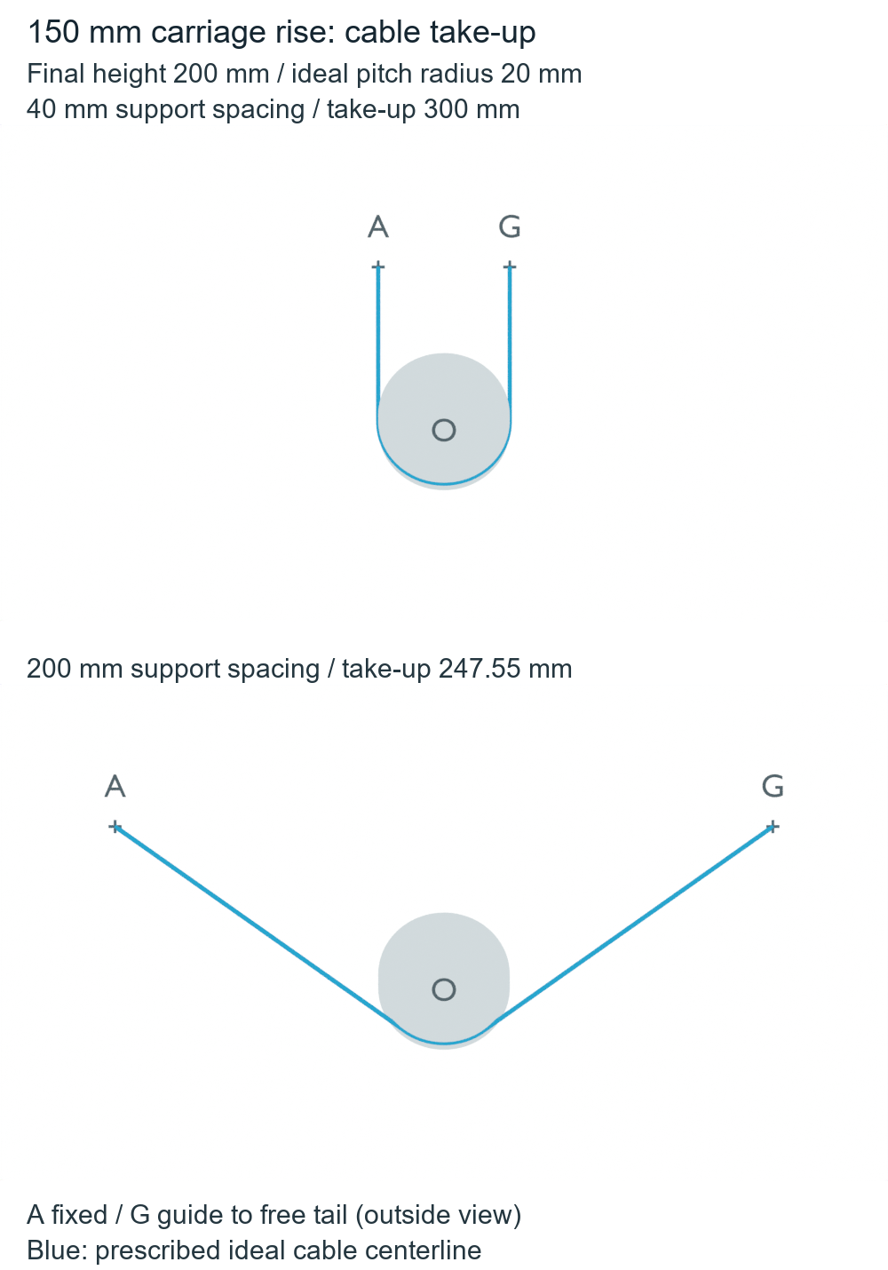
Map the complete chosen cable route over the carriage stroke before assigning a constant cable-to-travel factor. These are synthetic path calculations checked against finite Blender geometry; they do not measure force, efficiency or hardware behavior.
Define which cable length is allowed to change
The modeled cable runs from a fixed left anchor A, around the lower part of a moving pulley, to a fixed right guide point G. A free tail through G supplies cable or takes it in. The section between A and G can therefore change length. Fixing both cable ends permanently would impose a different constraint and would not permit the prescribed motion with an inextensible cable.
Use an ideal 20 mm cable pitch radius. Put A and G at the same height, 250 mm, and place the pulley center halfway between them horizontally. The center rises from height 50 mm to 200 mm, reducing its vertical distance below the support points from 200 mm to 50 mm.
For the parallel layout, A and G are 40 mm apart: their horizontal coordinates are −20 and +20 mm. The two tangent legs are vertical. Each shortens by exactly the carriage rise, while the lower semicircle keeps its length. Two legs shortening by 150 mm account for the 300 mm take-up.
Now place A and G at −100 and +100 mm, giving 200 mm separation. The straight sections are angled, and their tangent points move around the circular pitch path as the center rises. The wrapped arc changes length too. Counting two legs while ignoring those changes loses the cable-to-carriage mapping.
The manufacturer discussion of ideal pulley systems relates system ratio to the amount of rope pulled and distinguishes its ideal model from real pulley behavior. The finite-radius, spread-support numbers here are our own geometric calculations. They are not Petzl test results or instructions for a lifting system.
The ratio changes within one stroke
In the spread layout, the calculated local travel ratios are approximately 1.862, 1.777, 1.600 and 1.200 as the center-to-support height falls through 200, 150, 100 and 50 mm. The average over the complete 150 mm stroke is about 1.650. Neither that average nor a value measured at one position describes the entire mapping.
The calculation retains both straight tangent sections and the chosen lower circular arc. Let a be half the support spacing, d the vertical center-to-support distance, and R the pitch radius. The distance from the center to either support is D = sqrt(a²+d²), and each straight tangent has length sqrt(D²−R²).
The following standard-library code adds the changing arc and returns the local take-up ratio. Its selected layout uses a≥R and d>0. Distances are in meters internally; the printed take-up is in millimeters.
from math import hypot, sqrt, acos, atan2, pi

# Synthetic meters. Fixed support points at (+/-a,H); center at (0,H-d).
def length_and_ratio(a, d, R=.02):
    D = hypot(a, d)
    if D <= R:
        return None  # no nondegenerate straight tangent leg
    if a < R or d <= 0:
        return None  # outside this example's selected lower-wrap layout
    span = sqrt(D*D-R*R)
    phi = acos(R/D)-atan2(d, a)
    length = 2*span + R*(pi-2*phi)
    ratio = 2*(d*span+a*R)/(D*D)  # cable take-up per small upward center move
    return length, ratio

for name, a in [('parallel', .02), ('spread', .1)]:
    values = [length_and_ratio(a, d) for d in (.2, .15, .1, .05)]
    print(name, 'local travel ratios:', [round(v[1], 3) for v in values])
    print('150 mm carriage rise -> cable take-up mm:',
          round((values[0][0]-values[-1][0])*1000, 3))
assert abs(length_and_ratio(.02, .1)[1]-2) < 1e-12
assert length_and_ratio(.02, 0) is None
assert length_and_ratio(.01, 0) is None
The sign convention matters: upward motion reduces d and reduces the cable length between A and G. Take-up over a stroke is the starting path length minus the ending path length. The ratio in the code is the positive local amount taken in per upward center displacement; it is not an experimentally measured force multiplier.
Check the circular path separately from its drawing
The AI-operated Blender 5.2.2 LTS study on October 5, 2026 used a 96-sided finite disk to locate the pulley and a sampled cable centerline with 64 intervals on the arc. Straight chords slightly underestimate the smooth circular arc. An outer tangent polygon provides an upper bound, allowing the finite drawing and the ideal circular calculation to be compared without claiming that the polygon facets are the contact surface of a real pulley.
An independent audit recovered the center from paired disk vertices and the radius and plane from finite landmarks. A separate point-to-circle tangent construction checked all evaluated vertices, topology, perpendicular straight legs, the positive lower arc and direction-based travel ratios. Ten static records produced eight valid paths and two invalid controls, using twenty-eight meshes. The actual reconstructed circular-path take-up was approximately 299.999779 mm for the parallel layout and 247.549451 mm for the spread layout, agreeing with the rounded explanation.
For a stroke difference, the lower bound subtracts the ending upper path length from the starting lower path length; the upper bound does the reverse. Actual finite bounds were approximately 299.980847–300.018927 mm and 247.545801–247.555553 mm. Subtracting two chord lower bounds alone would not give a lower bound on the take-up. A support on the pitch circle has no nonzero straight tangent leg; a support inside it has no real tangent. Those controls retain no cable path or travel ratio. Other routes outside the selected layout are not declared impossible merely because this example does not construct them.
The audit used 4 μm for geometry, 5 μm for analytic path agreement and 0.00003 for angle/direction consistency. These are numerical guards, not physical cable accuracy. A proper common XYZ rotation of (15,−20,25)° and separate display translations were included in the finite readback; only those translations were removed for the final-height comparison. No cable equilibrium, contact, force, efficiency, controller, product or hardware test was run.
The right support is an ideal point guide. A real guide’s radius, its contact arc and the cable route beyond it can add further changes, so the reported take-up applies only to the stated section. Cable thickness, groove geometry, stretch, sag, tension and friction are also outside the model. The practical geometric check is to map the complete chosen path over the carriage stroke before assigning a constant cable-to-travel factor.
The robot actuator overview explains why remote cable and belt drives move actuator mass and introduce routing constraints. Here the narrower implementation choice is the cable-to-carriage mapping. For another route-dependent geometry question, the open and crossed belt study separates output direction, wrap and route intersection while keeping shaft centers fixed. Changing a moving pulley’s support spacing instead changes the travel mapping throughout its stroke.