Robot system identification estimates a mathematical model from commanded motion and measured response. For a manipulator, the target may include inertial combinations, gravity, friction, motor torque constants, transmission effects or flexible modes. The purpose is not to reproduce one log perfectly; it is to obtain a model that predicts useful behavior on new motion.
The workflow begins before regression. Coordinates, sensor meanings and actuator paths must be defined, then the robot needs safe trajectories that excite the terms of interest. Position, velocity, acceleration and torque evidence must share a time base. Estimation comes only after observability, noise and physical constraints have been considered.
Use this guide with the robot joint actuator test guide and inverse kinematics versus inverse dynamics guide. A low training residual is not evidence of an identifiable, physically plausible or transferable model.
Define the model before collecting data
Choose the input, output, state and reference frame that the model will represent. A rigid-body inverse-dynamics model maps motion and acceleration to joint torque, while an actuator model may map current to motor torque and include transmission loss. Flexible joints, cable forces and temperature-dependent friction require additional terms or an explicitly limited operating range.
Document units, sign conventions, gear ratios, payload, tool frame, controller mode and any compensation already active in the drive. Otherwise the estimated parameters can absorb hidden gravity, filtering or inner-loop behavior. A model identified from commanded current is different from one identified from measured output torque even when both use the word torque.

Not every physical parameter is separately identifiable
Robot inverse dynamics can often be written as a regressor multiplied by a parameter vector, but columns of that regressor may be linearly dependent for the available mechanism and measurements. Only combinations called base or identifiable parameters can then be recovered. Reporting every link mass and inertia as an independent measured truth overstates what the data contain.
Use rank, singular values and parameter covariance to find weak directions. Reparameterize or regularize only with an explicit prior, because a numerical answer does not create missing information. CAD values can supply a prior or fill unidentifiable terms, while the experiment estimates combinations that materially affect the measured dynamics.
| Model term | Evidence needed | Common confounder | Useful check |
|---|---|---|---|
| Rigid-body inertia | Varied acceleration and pose | Payload or frame error | Base-parameter rank |
| Gravity | Pose coverage | Joint zero offset | Slow pose sweep |
| Viscous friction | Both velocity directions | Back EMF or filtering | Speed sweep |
| Coulomb friction | Low-speed reversals | Stiction and hysteresis | Direction comparison |
| Actuator gain | Independent torque reference | Transmission efficiency | Load-cell calibration |
Design excitation for information and safety
An identification trajectory should vary joint position, velocity and acceleration enough to separate the selected terms. Multi-sine or Fourier-series trajectories are common because bandwidth and amplitude can be controlled. The exact design must respect joint, velocity, acceleration, current, torque, collision and workspace limits throughout the robot, not only at sampled waypoints.
Optimize an information measure such as a regressor condition metric, then simulate the candidate trajectory using conservative limits. Begin at reduced speed and energy, monitor tracking and abort conditions, and preserve clearance for calibration error. More aggressive motion is not automatically more informative if it saturates the drive or excites unmodeled flexibility.
Synchronized measurements determine usable bandwidth
Timestamp position, current, torque and external sensors at their physical sampling points when possible. Constant delay can rotate phase and bias inertia or damping estimates; variable delay broadens the error. Resampling does not restore information lost to an unknown acquisition pipeline. Measure clock relationship and log sequence gaps.
Velocity and especially acceleration derived from encoder position amplify quantization and noise. Choose filtering and differentiation together with the motion bandwidth, and account for their delay. Compare measured velocity when available, a smoothed derivative and an estimator-based derivative. Report filter cutoff and phase behavior so the identification can be reproduced.
Separate rigid-body torque from actuator effects
Measured motor current passes through torque constant, transmission ratio, efficiency, friction and controller behavior before it represents joint output torque. Friction can depend on direction, speed, temperature, preload and dwell. A single Coulomb-plus-viscous model may be adequate for one operating band but biased around reversal or warm-up.
Run dedicated low-speed and bidirectional tests to expose friction asymmetry, then decide which effects belong in the plant model and which remain in residual uncertainty. Keep current-loop saturation, gravity compensation and feedforward logs. A parameter estimate that silently includes an active compensator will fail when that compensator changes.
| Data problem | Effect on estimate | Detection | Mitigation |
|---|---|---|---|
| Clock offset | False damping or inertia | Cross-correlation and timing test | Hardware timestamps |
| Acceleration noise | High torque residual | Spectrum and repeat runs | Bandwidth-aware derivative |
| Current saturation | Clipped actuator gain | Drive status and command gap | Reduce excitation |
| Thermal friction drift | Run-order bias | Temperature trend | Warm-up and stratify |
| Payload mismatch | Wrong inertial terms | Configuration comparison | Record tool and load |
Use constrained estimation when physical meaning matters
Ordinary least squares is a useful baseline when noise is mainly in torque and the regressor is well conditioned. Weighted least squares can represent channel variance, while robust losses reduce the influence of isolated outliers. If motion variables are noisy, errors-in-variables effects need consideration rather than assuming the regressor is exact.
Physical consistency constraints prevent impossible inertial combinations such as negative mass or invalid inertia tensors. Research on fully physically consistent inertial identification shows why a plausible rigid body imposes more structure than element-wise bounds. Constraints should be reported with the objective and solver; they do not compensate for weak excitation.
Residual structure reveals missing dynamics
Plot residual torque against time, joint position, velocity, acceleration, direction, temperature and commanded load. White, small residuals are encouraging, while periodic, sign-dependent or pose-dependent patterns point to cogging, friction, calibration or kinematic errors. A single root-mean-square value hides these diagnostic relationships.
Check cross-joint residual correlation and frequency spectra. A flexible mode can create a narrow frequency peak even when average error is low. Repeat the same excitation to estimate measurement variability. If residuals change after warm-up, include temperature in the model or state a thermal envelope instead of averaging incompatible runs.
Validate on motion not used for fitting
Reserve trajectories, payloads or speed bands before fitting. Use the identified model to predict torque or forward response without adjusting parameters on that test set. Compare against a simple baseline such as CAD parameters or gravity-only compensation so improvement has a meaningful reference.
Held-out validation should include interpolation within the intended envelope and deliberate boundary cases. Report mean, percentile and worst residual, plus task-relevant effects such as tracking improvement or simulator prediction. Cross-validation over adjacent samples from the same trajectory can be misleading because those samples are strongly correlated.
Model quality depends on the intended use
An inverse-dynamics feedforward model may tolerate errors that would destabilize a high-bandwidth observer. A simulator needs forward dynamics, contacts and actuator limits that a gravity compensator does not. State the downstream purpose, update rate and acceptable prediction error before choosing model complexity.
For deployment, compare the model with the joint gain-tuning workflow and collision-detection guide. Keep feedback stability and protection independent of optimistic model accuracy. Identification improves a controller input; it does not certify the complete motion system.
A reproducible package includes evidence
Archive the robot description, payload, firmware, controller gains, estimator code, calibration, trajectory generator, raw timestamps and unmodified sensor logs. Store the fitted parameter basis and transformation back to any reported physical quantities. A parameter table without its regressor definition cannot be independently interpreted.
Recent work on physically consistent identification in robot contact illustrates that measurement choice and structural assumptions remain central even as optimization methods change. Publish training and validation splits, residual plots, parameter uncertainty and known exclusions so another team can judge transfer.
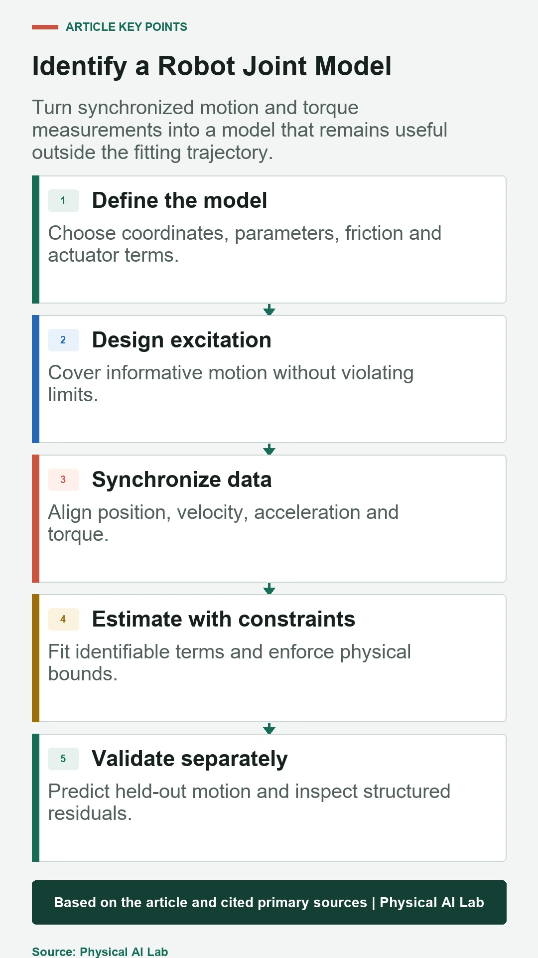
- Define coordinates, actuator path and compensation state.
- Design informative trajectories within verified limits.
- Synchronize and preserve raw measurements.
- Estimate only supported parameter combinations.
- Validate on held-out motion and publish residual evidence.
Frequently asked questions
Can one trajectory identify every robot parameter?
Usually not. Identifiability depends on mechanism, sensors, model and excitation. Estimate supported base-parameter combinations and state which terms came from priors.
Should CAD parameters be discarded?
No. CAD is a useful baseline and prior, especially for weakly observable terms. Measured identification can refine combinations that affect the operating robot.
Why does acceleration filtering change the result?
Differentiation amplifies encoder noise, while filtering adds attenuation and phase delay. Both change the inverse-dynamics regressor and therefore the fitted parameters.
Does a low fitting error prove a correct model?
No. Overfitting, delay, hidden compensation and correlated data can all create a low training residual. Held-out prediction and residual structure are required.
When should the robot be reidentified?
Recheck after payload, transmission, lubrication, sensor, firmware or controller changes, and when residual trends show temperature or wear outside the validated envelope.
System Identification Evidence Boundary
System identification estimates a model under stated sensors, excitation, configuration and operating conditions. Preserve independent feedback limits and validate any control or safety use on the complete robot.