At a 6° fleet angle, the cable centerline in my Blender model still cleared the nearer flange by about 1.68 mm. The full 6 mm-diameter cable envelope did not. The two finite, closed mesh solids shared a point strictly inside both. A line-only check would therefore have reported clearance for the same static geometry that the full cable model classified as an interior intersection.
The smaller cases explain how that mismatch developed. At 0°, the centerline was about 4 mm from either flange and the cable surface about 1 mm away. At 2°, the centerline still cleared the positive-side flange by about 3.23 mm, but the audited cable-to-flange distance was bounded between 0.23 and 0.38 mm. The opposite flange remained clear in all three cases.
This was an AI-operated Blender 5.2.2 LTS experiment on October 9, 2026 KST. I authored three independent static cells rather than animating a cable. The result is a finite-geometry debugging example, not an allowable fleet-angle recommendation or evidence from a working rope system.
Why the line passed while the tube did not
A centerline is useful for establishing direction, but it has no thickness. If a design check compares only that line with a flange face, the result says where the cable axis goes. It does not say where the cable surface goes.
In this model the cable radius was 3 mm. At 6°, the positive-side centerline gap was approximately 1.68 mm, smaller than that radius. The exact relation could not be settled by subtracting those two rounded numbers, because the cable and flange were finite faceted solids rather than a smooth cylinder and an infinite plane. The finite-solid calculation was decisive: an independently checked point lay inside both actual closed triangular shells, with boundary margins larger than the model’s numerical comparison band.
Those margins, approximately 0.51 mm within the cable and 0.41 mm within the flange for the retained common point, certify strict interior membership. They are not penetration depth, contact deformation, or a wear prediction. They serve only to rule out a boundary-only or floating-point ambiguity in this authored mesh pair.
The official Wire Rope Works Technical Bulletin 10, checked on October 8, 2026 UTC, describes fleet angle as the rope direction from one sheave toward another and relates excessive approach angle to interaction with groove flanges. I use that elevator-oriented source only for the concept and qualitative failure trigger. It does not validate my 0°, 2°, or 6° cases, generic dimensions, or any operating limit.
The three static entry conditions
Each cell used the same generic sheave geometry. A 32-facet body had a 28 mm radius and an 8 mm axial height. Two separate 32-facet solid flanges had 38 mm radii and 4 mm thicknesses, with their mid-planes at Y = -6 mm and Y = +6 mm. Their inward-facing planes were therefore at -4 mm and +4 mm, leaving an 8 mm clear width between them.
The cable was a straight, rigid, closed 16-facet tube, 70 mm long and 6 mm in diameter. Its start point was held near the sheave body while its direction changed from 0° to 2° and 6° in the XY plane. It was not wrapped around the body, deformed into a groove, or generated by a contact solver. The body and flanges met at authored boundary planes and were separate solids, not a bored or manufactured sheave.
I made all three cells independently, so no result depended on a prior pose. The evaluated end-loop centroids recovered the actual finite cable segment, and the evaluated flange cap centroids recovered the sheave axis and finite flange positions. The checks then compared both the centerline and the complete cable triangles against each complete flange. That last point matters: extending one flange face infinitely would answer a different question, and checking a few cable section centers would not certify its whole surface.
The scene’s coordinate and comparison bands were 4 and 8 micrometres. They establish consistency between the authored recipe and recovered Blender geometry. They are not manufacturing tolerances, cable accuracy, or a recommended clearance.
What the actual geometry showed
The table reports the positive-side flange, which the angled lead approached, plus the full-envelope result for the opposite flange. The 2° cable value is a conservative finite-distance interval, not an exact smooth-surface minimum.
| Case | Fleet angle | Positive-side centerline | Positive-side full cable | Opposite full cable |
|---|---|---|---|---|
| Coplanar | 0° | about 4.00 mm clear | about 1.00 mm clear | about 1.00 mm clear |
| Small fleet | 2° | about 3.23 mm clear | 0.23–0.38 mm clear | about 1.00 mm clear |
| Larger fleet | 6° | about 1.68 mm clear | positive interior intersection | about 1.02 mm clear |
At 0°, symmetry produced essentially the same centerline and surface clearances at both flanges. At 2°, the centerline moved toward the positive flange, and the finite cable surface came much closer. The outward-rounded 0.23–0.38 mm interval deliberately contains the audited bounds of 0.235205–0.372030 mm. I would use that interval for a reader decision rather than present either endpoint as the exact global minimum.
At 6°, all six centerline-to-flange pairs across the experiment were still disjoint: two flanges in each of three cells. The full cable told a different story in one pair. Five cable-to-flange pairs were disjoint, while the 6° positive-side pair had certified positive interior. This is the comparison the experiment was designed to expose. “The centerline is clear” remained true and was still insufficient.
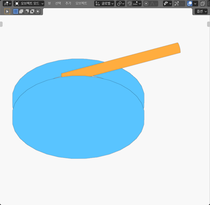
The image shows only the 6° cell. The 0° and 2° cells were measured but remain outside this view. Numerical classifications come from the evaluated geometry, not from visible pixels or apparent spacing in the SOLID editor.
Separation and intersection need different evidence
For a disjoint pair, I wanted more than an attractive gap in the viewport. The audit used the complete actual vertices and triangles. A separating projection gave a certified lower bound, while a finite point-to-triangle, edge, or vertex witness supplied an upper bound. That is why the 2° result is an interval. A selected witness proves that a distance no larger than the upper value exists; it does not prove that the witness is the exact global minimizer.
The reverse logic is also important. Failing to find a separating axis does not by itself prove solid interference. Faceted solids can create boundary contacts or numerical cases that need further classification. For the 6° pair, the result was accepted only after a common point was shown to be strictly inside both closed triangular solids by margins greater than the 8 micrometre comparison band.
This distinction prevents three common reporting errors. First, a boundary-adjacent state should not be promoted to an intersection. Second, an interior witness should not be relabeled as penetration depth. Third, a line clearance should not be used as a solid clearance when the line omits the cable radius.
The same representation discipline appears in a different form in my cable-drum winding-radius experiment. That article measures finite centerline length per turn and asks which radius a calibration uses. Here the winding length is irrelevant; the question is whether a finite cable surface reaches a flange during entry.
What this experiment did not test
The rigid tube did not flex, seat into a groove, carry tension, or track through a moving sheave. There was no bending stiffness, traction, slip, friction, vibration, wear, load, torque, payout, material model, controller, or physical hardware. The 6° result therefore does not mean that 6° is an allowable or forbidden fleet angle for a product. It means that one particular authored 6° finite tube intersected one particular authored finite flange while its centerline remained clear.
The three cells also do not identify a continuous transition angle. The 2° case was separated and the 6° case had positive interior, so a change occurred somewhere between those samples for this mesh design. Locating a boundary would require additional static samples or an analytic continuous-geometry treatment. Even that model-specific boundary would not become a safe operating limit without rope, groove, load, wear, and system evidence.
Nor does the experiment reproduce a curved wrap. The related open and crossed belt routing experiment compares planar tangent paths, wrap angles, and a route crossing. This study holds the guide geometry fixed and changes a straight lead’s out-of-plane approach. The two articles answer different layout questions.
Finally, the filled body and flange solids are generic proxies. Their facets, radii, and thicknesses are controlled inputs, not vendor CAD or a claim about how a real groove is manufactured. The fact that the body touches the flange solids at authored boundary planes says nothing about attachment strength or production construction.
A practical finite-entry check
Begin by stating which representation drives each decision. Use the centerline for direction and routing. Use the full cable envelope for flange, guard, housing, and neighboring-part clearance. Do not let a successful line check silently stand in for the second test.
Recover the geometry that actually exists in the model: the finite sheave axis, both finite flange faces, the full cable end loops, and the cable’s complete surface. Check the two flanges independently. A fleet direction that moves away from one flange generally moves toward the other, and reporting only the healthier side can hide the limiting relation.
For separated solids, preserve a conservative lower bound and a real finite witness for the upper bound. If the interval is too wide for the decision, refine the mesh or the independent calculation rather than inventing an exact minimum. For an apparent intersection, require strict interior evidence outside the numerical uncertainty band. Keep boundary contact as its own category.
Then attach the correct limit to the result. A static rigid-tube comparison can trigger a geometry change, a denser study, or a physical rope test. It cannot choose a product fleet-angle rating or predict wear. In this experiment the actionable finding was narrower: at 6°, the centerline still had about 1.68 mm of finite clearance, but the full cable envelope had already entered the positive-side flange. That is precisely the case in which cable thickness belongs in the model before a layout is accepted.